My Into Depth project is still fairly small, in the grand scheme of things. I’ve authored about 17k lines of code, which you’d think would compile pretty quickly, but I was seeing clean compile times of about 40 seconds. That is too long.
Sure, I’m not just compiling the code I wrote. glad, glm, imgui, and stb increase the line count by about an order of magnitude to 120k. However, 40s is 40s, and I wanted to see what I could do to reduce it.
Problems
There are fundamentally two problems here – long full compilation times and long incremental compilation times. A full compilation happens after, e.g., make clean, where everything is compiled fresh. This naturally takes longer, since all object files have to be generated. An incremental compilation is what happens most of the time, where you have an existing set of object files and just need to recompile one or two of them and re-link.
The Compilation Process
To understand how we’re going to speed things up, its helpful to understand what, roughly, is happening in the first place.
The Preprocessor
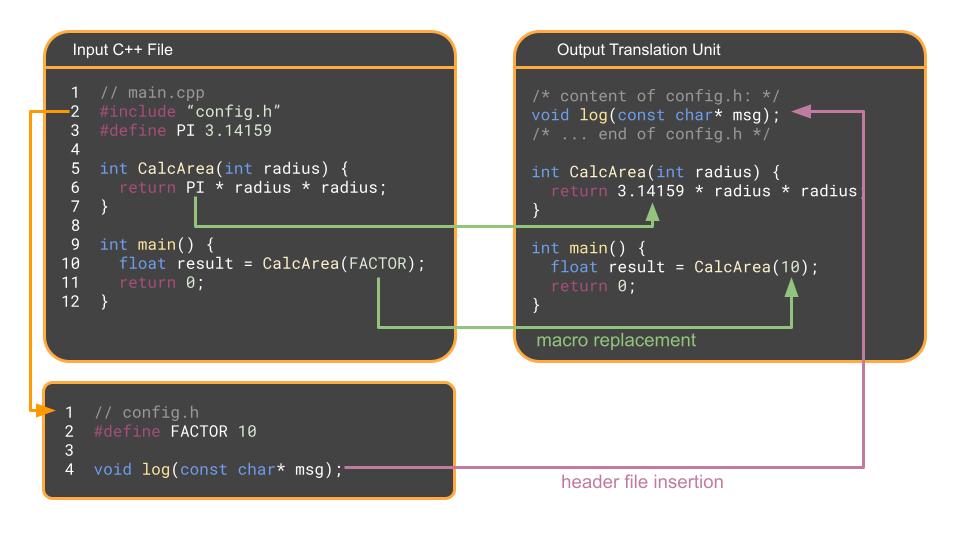
The first stage, before any compiling happens, is where the preprocessor runs over each .cpp file and specifically handles # commands. The preprocessor doesn’t actually understand C++ syntax, but is more of a glorified find and replace tool.
It finds every #include and copy-pastes the contents of that header file into the .cpp file.
It finds every #define, i.e., macro, and replaces it with the corresponding text.
It strips out all comments.
The result is a massive, single file of pure C++ code called a translation unit. For a standard codebase where your C++ file has many inputs, the translation unit can be pretty large.
The Compiler
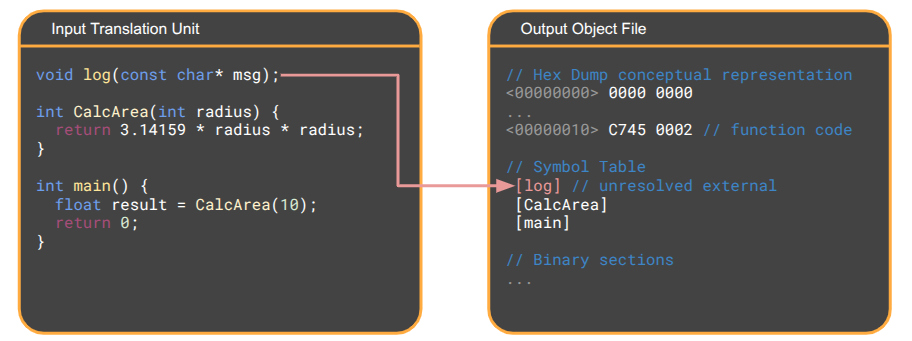
The compiler translates the C++ code in each translation unit into raw machine code – the binary instructions that your specific CPU understands – as an object file. On Linux/Mac, these are .o files, and on Windows these are .obj files.
Object files contain:
A header
a code segment with the binary instructions for the functions defined in the translation unit
a data segment with initialized static variables
a read-only data segment with initialized static constants
a section for uninitialized static data (e.g., int stuffs[1000000];)
A symbol table listing the functions and variables that this translation unit can offer to others.
A set of unresolved references that the object file expects to exist but doesn’t have just yet – functions or global variables it needs from other object files.
Debugging information.
Concepts like structs only matter during the compilation phase, where they inform the compiler how much memory to allocate on the stack or what offsets to look at variables for. The resulting object files only care about memory addresses, function blocks, and global variables.
The Linker
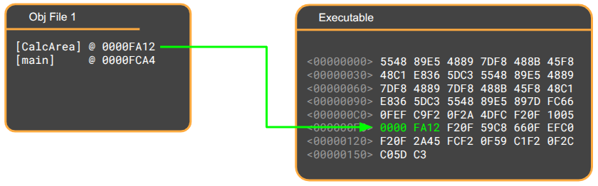
Once all of the .cpp files have been compiled into a bunch of .obj files, the linker will handle the task of resolving references. If an object file needs a reference that the linker cannot find, it will issue the undefined reference or unresolved external symbol errors we know so well. Similarly if it finds multiple object files offering the same function signatures, it will output a multiple definitions error.
When building a executable (as opposed to a library), the linker starts by creating a new, empty file on disk (e.g., game.exe). This file has an OS-specific format, such as ELF on Linux and PE on Windows.
Next, the linker reads every .obj file and copies the machine code binary into the executable, stacking them into one large, contiguous section.
Each object file listed its unresolved symbols, along with where, in its compiled code block, the address of the symbol should be written once the symbol is finally resolved. The linker thus works through the copied binary sections and writes the appropriate jump instructions to jump to the right function calls or load the right global variable address. This process is called relocation.
The linking step also handles any libraries that your executable depends on. Any static library (.a for ‘archive’ file on Linux, .lib on Windows) is basically a collection of object files, and is copied into your executable like the other objects. Any shared library (.so file on Linux, .dll for ‘dynamic linked library’ on Windows) is not copied, but the linker instead records a reference to it in the executable that the dynamic linker connects when your OS goes to execute your file.
Once the linker has completed relocation, it is done, and game.exe is a self-contained block of machine code (except for references to dynamic libraries). You can actually delete all of the .obj files and the executable will work just fine. The primary reason .obj files are kept around is for incremental builds.
Faster Clean Builds
Now that we have an understanding of the compilation process, we can reason about changes that will speed up compile time. The first such speedup will be for clean builds, which is a complete build that runs the entire compilation pipeline without using any cached work.
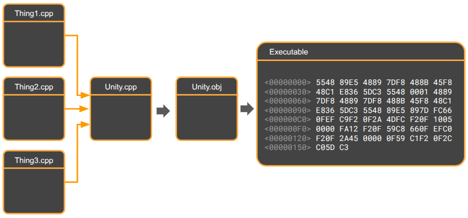
Under a typical build structure, many object files are produced and then linked:
The trick here is the unity build, which collapses the project’s many object files into just one:
This is achieved by creating a .cpp file that includes all of the project’s other .cpp files, and then only have our Makefile build that one target.
In practice, the linker still needs to do some work. Most code bases will still link against libraries, and it is recommended to compile external dependencies that we do have the source for into separate .obj files and link against them.
Time is saved in the linking phase by not having to stitch together potentially thousands of small object files. All of the memory math is handled by the compiler, which has access to all of the definitions.
The primary time savings typically comes from eliminating redundant header parsing. In compilation, each translation unit receives copies of the headers it includes. The same header, such as <vector>, may be used in many translation units, and will be repeatedly parsed for each one. Having a single translation unit allows the #pragma once guards to do their work and ensure the preprocessor only copies each header once, so each header is only parsed once.
Unity builds also benefit from being able to do more inlining, as methods across translation units either cannot be inlined, or require link-time optimization to be enabled, which makes linking that much slower. In a unity build, everything is in one object file, so the entire program can be optimized.
The final speedup comes from reduced disk I/O. The compiler does not need to repeatedly read header files or write many object files.
Moving to a unity build dropped clean build times for ~45s to under 5s!
Faster Incremental Builds
During typical development, code is rebuilt incrementally. Here, a full build has already happened, you edit one or two .cpp files, and run make again. In an incremental build, only the .obj files for the two edited .cpp files need to be recompiled, followed by linking.
Using a unity build means changing a single .cpp file requires the compiler to do the full work of producing the one .obj file all over again. As such, large projects will tend to use standard builds for typical development and unity builds for release builds or CI/CD pipelines.
We can use another technique to speed up incremental builds. Here, we aim to reduce the time it takes to compile individual object files.
Time can be saved by reducing the work done by the preprocessor in copying header files included in other header files by using forward declarations instead.
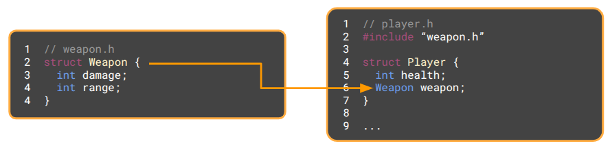
Consider the following example, where a Weapon struct is defined in weapon.h and it is used by a Player struct in player.h:
If we later change Weapon, such as by adding a new int cooldown, and go to compile, the build system will see that weapon.h has changed. The player.h file includes weapon.h, so it is marked for recompilation and any file that includes player.h is also recompiled. A simple field change has cascaded into a large number of updated object files.
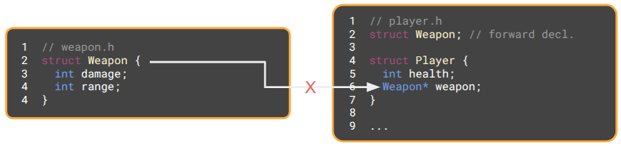
As written, player.h must include weapon.h, because Player contains a Weapon, and the compiler needs to know its size. We can avoid this dependency by using a pointer instead. The compiler cares about memory layouts, and pointers are all the same size, so we can use a forward declaration to promise the compiler that Weapon exists somewhere and avoid including weapon.h:
Now, if Weapon is changed, player.h is completely unaffected. Any .cpp files that merely include player.h no longer need to be recompiled.
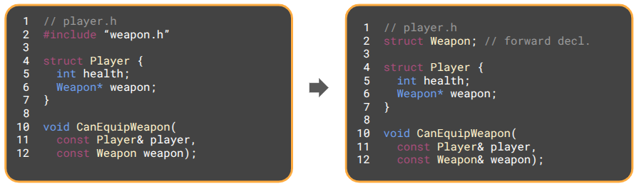
The same trick works for methods as well. Passing a struct like Weapon by value will require knowing its size. Changing to a pointer or reference (which is basically a pointer) removes that requirement, and a forward declaration is enough to promise that the type will eventually be defined.
The Best of Both Worlds
We can get the benefits of both unity builds during full recompilation and forward declarations during incremental builds by modifying our Makefile to run a default incremental build when make is involved and have a separate command, make unity, that compiles unity.cpp directly into an executable:
# --------------------------------------------------------- # TARGET 2: The Unity Build # --------------------------------------------------------- # Notice this target does NOT depend on $(OBJS). It bypasses them. unity: src/unity.cpp $(CXX) $(CFLAGS) src/unity.cpp -o $(TARGET) $(LDFLAGS)
This sort of a setup is not quite a panacea – you must suffer the cost of a full non-unity build in order to take advantage of incremental builds. As such, I’m personally going with all unity build, all the time for now (something Casey Muratori has espoused). Clean files seem safest.
It is worth mentioning that unity builds also prevent repeated definitions using the same function name. Any nameless namespaces or static helper functions in your .cpp files all get merged together, hence a chance for collision.
Conclusion
Overall, I found this foray into compilation time quite satisfying. Not only did this process reduce how much time I sit around waiting for code to recompile, it also forced me to better understand the whole C++ compilation process. Oftentimes, a basic understanding of the system can make a huge difference in making informed decisions and understanding what the compiler is trying to tell you when something goes wrong.
Mykel Kochenderfer and I are finishing up the second edition of Algorithms for Optimization with MIT Press. The first edition took about five years, and the second edition has *only* taken… another five years. You can read it here.
What started as a simple extension with three new chapters became much more extensive. We overhauled many existing chapters, added new sections to others, and generally touched up the entire book. It has earned the title of second edition.
Modern technical textbooks include alt text, which are short annotations attached to images that allow visually impaired readers to receive those descriptions via screen readers. MIT Press authors provide alt text for every graphic element by submitting a spreadsheet in addition to the manuscript. Having alt text definitions live in a different place than our LaTeX source immediately felt like a bad idea. We don’t want to rely on memory to keep the alt text document up to date every time we change a figure or introduce a new one.
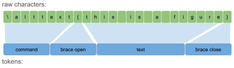
I decided very early on that I wanted the alt text descriptions to be alongside each graphical element in the LaTeX source. I defined a macro, \alttext{...}, and use that in every graphical element:
\begin{marginfigure}
    \centering
    \begin{tikzpicture}[
    	->, >=stealth',
    	level/.style={sibling distance = 1.5cm/#1, level distance = 1cm},
    	mynode/.style={circle, minimum size=7mm, align=center},
    	terminal/.style={mynode, draw=black, fill=none},
    	nonterminal/.style={mynode, draw=pastelBlue, fill=pastelBlue},
    	]
    	\node [terminal] {$+$}
    	child{ node[terminal] {$x$} }
    	child{ node[terminal] {$\ln$}
    		child{ node[terminal] {$2$}
    		}
    	};
    \end{tikzpicture}
    \alttext{A directed acyclic graph with a root plus node, a left-side x node, and a right-side natural log node with a two-node child.}
	\caption{
        \label{fig:expr-ln}
        The expression $x + \ln 2$ represented as a tree.
    }
\end{marginfigure}
These annotations let us update the alt text any time the figure is changed. The macro evaluates into nothing (\newcommand{\alttext}[1]{}), so it doesn’t affect document compilation. Great!
Unfortunately, MIT Press still needed a spreadsheet containing the figure numbers, captions, and their corresponding alt text. I needed an automated way to export the alt text annotations from the LaTeX source.
The First Attempt: Per-Line Scanning
My initial approach was to write a Julia script that scanned each LaTeX source file line-by-line and used regex matching to identify graphical elements and the \alttext macros. This script served a few purposes. First, it could identify which graphical elements still lacked alt text entries. Second, it allowed us to automatically check that our alt text entries adhered to MIT Press standards, such as avoiding certain characters and staying below a length limit. Finally, it packaged them up and exported the data to the required spreadsheet.
The first challenge was figure identification. The script looked for environments like \begin{tikzpicture} and commands like \plot. Unfortunately, there was more nuance here than one would have initially thought. TikzPicture environments can be nested, and in a few cases we define a new command containing a TikzPicture environment, only to invoke it later with a \protect to inject it safely into a caption. We also have \begin{ignore} environments, and have to ignore graphical elements in those.
After graphical elements were identified, I searched within them for an alt text entry. This was done with a simple lookahead search. Not ideal, but it worked fairly well.
function find_alttext(lines, line_index_lo::Int, line_index_hi::Int)::String
    for line in lines[line_index_lo:line_index_hi]
        m = match(r"\\alttext\{([^}]+)\}", line)
        if isa(m, RegexMatch)
            return strip(m[1])
        end
    end
    return ""
end
MIT Press wanted the figure numbers for each alt text entry. That is, if a figure has a caption with, e.g., “Figure 5.7”, we wanted 5.7 exported in the spreadsheet. LaTeX does all of the numbering at compile time, which is extremely convenient, but that makes it harder to infer from the source. The script had to keep track of figure numbers, incrementing them over time, but only for graphical elements that had such captions. The script would try to figure out whether a caption existed, but would only assign a new figure number if the graphical element was actually a figure or margin figure.
This script was used for the first version of the spreadsheet that we sent to MIT Press. It worked really well with respect to identifying figures that didn’t have alt text, and verified the content of the entries. Unfortunately, it did have some issues with figure number identification, and I ended up having to manually scan through all figures in the book and manually update the spreadsheet – exactly what I had wanted to avoid doing.
A Better Way: Lexing and Parsing
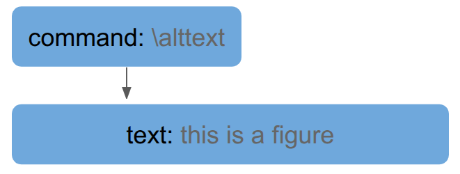
LaTeX source code is, well, code. And code is fundamentally hierarchical. Thinking of source code as a list of lines has a lot of downsides. Instead, to extract the data accurately, the script needed to understand the structure of the document more like the LaTeX compiler does. I started over, writing a proper lexer and parser, thereby providing a simple Abstract Syntax Tree (AST).
A lexer’s job is to convert the source code – a long bytes array – into a sequence of manageable tokens. Reasoning about a character sequences like "\alttext{this is a figure}" is a lot harder than reasoning about <command><brace_open><text><brace_close>.
Each Token is effectively an enum that applies to a range of characters:
@enum TokenKind begin
    TOKEN_TEXT        # Raw text content
    TOKEN_COMMAND     # A LaTeX command starting with \, e.g. \alttext
    TOKEN_BRACE_OPEN  # An opening curly brace {
    TOKEN_BRACE_CLOSE # A closing curly brace }
end

struct Token
    kind::TokenKind
    i_byte_lo::Int
    i_byte_hi::Int
end
The next step, parsing, does the work of relating tokens to one another to form a tree. For example, in the running example, the text is an input into the \alttext command, so it becomes a child:
This tree lets us represent larger structures more efficiently. For example, the marginfigure code sample at the top ends up being represented as a tree:
This tree structure makes it much easier to tell whether a caption is defined for the margin figure, or whether there is an alt text command, or whether the marginfigure itself is inside an ignore environment.
Nodes are more complicated than Tokens, but not by much:
@enum NodeKind begin
    NODE_ROOT    # The root node of the abstract syntax tree (AST)
    NODE_TEXT    # A text node
    NODE_GROUP   # A group of nodes enclosed in curly braces
    NODE_COMMAND # A command node, optionally with arguments as children
    NODE_ENV     # An environment like \begin{...} ... \end{...}
end

struct Node
    kind::NodeKind
    i_byte_lo::Int      # index into the original byte array of the first byte corresponding to this node
    i_byte_hi::Int      # index into the original byte array of the last byte corresponding to this node
    i_token_lo::Int     # index into the tokens array of the first token corresponding to this node
    i_token_hi::Int     # index into the tokens array of the last token corresponding to this node
    i_name_lo::Int      # index into the original byte array of the first byte of the command name
    i_name_hi::Int      # index into the original byte array of the last byte of the command name
    i_parent::Int       # parent node index, or zero otherwise
    i_first_child::Int  # first child node index, or zero otherwise
    i_sibling_next::Int # first sibling node index - circular list
    i_sibling_prev::Int # previous sibling node index - circular list
end
It supports five types of nodes. A true LaTeX compiler would of course do more, but we only need these. The root node is the root of the abstract syntax tree for the file being processed. Text nodes are basic text. Group nodes are formed from nodes enclosed by curly braces. Command nodes are commands like \alttext. Environment nodes represent a \begin{the_env}...\end{the_env} pair.
Using an AST made the alt text export logic much cleaner and more robust. This helped with the numbering issue, as it was easier to detect when a caption was defined, and whether a graphical element was inside an example or table.
We were able to detect when a graphical element was defined inside a \newcommand call, and added some basic tracking to find invocations of the defined command (typically after \protect). These deferred macros were really hard to do with the previous system.
Conclusion
Yay! We built a mini-compiler to avoid filling out a spreadsheet. That might sound wasteful, but for a five year project, spending a few days to ensure long-term maintainability is an easy decision.
What started as a simple string-matching script evolved into a LaTeX AST parser. Using the right data structure for the problem at hand made the exporting task a lot simpler. This process overall gives us the best of both worlds – our alt text lives next to the LaTeX for the graphical elements and it can be automatically exported into the spreadsheet that our publisher needs.
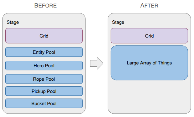
A depiction of the change in the data structure used to represent game entities, going from type-specific lists with a top-level entity table to a single large array of things.
Last month was a big overhaul of the underlying grid representation in order to be able to handle portals. This month ended up being another major refactor, but instead of the grid, I overhauled how game entities are stored.
I wanted to get Pickups back into the game in order to get the fundamental game loop: Heroes enter levels, gather Pickups, and exit to unlock items that make them more powerful. Once Pickups were working, I wanted to add other core mechanics like ropes (for climbing) and buckets (which hold Pickups and can be hoisted via ropes).
All of this logic made it very clear that my current way of interacting with entities was too cumbersome. I had a top-level Entity type that could be looked up by any entity’s ID, and then would itself contain a type enum and a type-specific ID in order to look up the specialized data in the type-specific list. That looked something like:
After this change, there is no indirection. All entities are in a single array:
// Grab the hero.
const StageThing* thing = Get(stage.things, entity_id);
ASSERT(thing.type == EntityType::HERO);
// Now we can directly access `thing.hero` and do stuff.
Making the transition to a Large Array of Things' data structure removed this annoying indirection. More importantly, it simplified how concepts are shared across entities (e.g., all StageThings now have a cell index). That shared context streamlined my event system - an AttachTo event no longer needs special logic for buckets vs. ropes vs. heroes – and drastically simplified my undo/redo system.
With this new architecture, I was finally able to implement some basic gameplay:
This video shows the state of the game at the time of writing. We see the rope being equipped before entering a basic level. The knight then deploys the rope, which the sorceress can then use to climb down, pick up a relic, and then climb back out. Graphics and UI are very rough first passes.
The rest of this post will cover why I used the original approach, what the Large Array of Things is, and how it led to these improvements.
Old Method: Type-Specific Lists
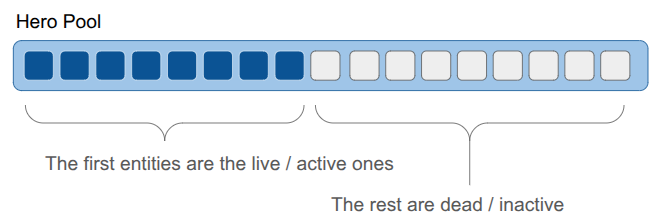
I started with type-specific lists for every entity type in my game, following what I understood was Billy Basso’s approach on Animal Well. Every entity type gets a struct, and we maintain an array of each struct type that has some max capacity, and we keep the array densely packed as entities are added or removed:
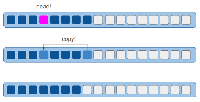
Keeping the live entities packed in the front makes iteration over the entities really fast. We only need to iterate over the first N elements, and they are all sequential in memory.
However, keeping the entities packed means that if an entity is deleted, we will move other entities around:
The result is that we can’t reliably point to an entity with a pointer, since its location in memory can change. To solve this, each ObjectPool maintained an extra layer of indirection. Each entity was referred to by an ID, which indexed into a lookup table to find the struct’s actual array index. All of this was managed internally by the pool, so the user never had to track it. I didn’t find this problematic at all.
At the beginning of game development, I was iterating through my lists of types quite a lot. Rendering was effectively:
for (hero in heroes) {
    RenderHero(hero)
end
for (rope in ropes) {
    RenderRope(rope)
end
// etc.
That approach was fine before I introduced portals. Now, the same tile might show up in multiple places on the screen. I was no longer able to just loop through the entities to render them; the entities themselves didn’t know where their cells were located in the final view. The iteration had to go the other way:
for (x in view.lo.x to view.hi.x) {
    for (y in view.lo.y to view.hi.y) {
        cell = grid.cells[x][y]
        for (entity in cell) {
            RenderEntityAt(entity, x, y)
        }
    }
}
With spatial iteration taking over, the primary benefit of densely packed lists completely disappeared. Yet, I was still paying the cost of indirection—which, honestly, was more about code line-count overhead than runtime performance—every single time I accessed an entity.
Old Method: Top-Level Entity List
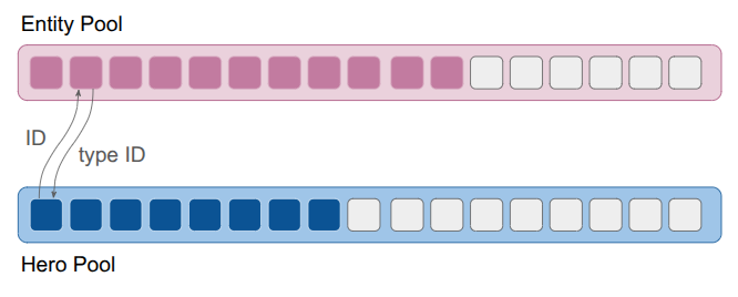
The type-specific lists were not sufficient when it came to entities referring to other entities. For example, a rope might refer to the entity holding it. Initially, maybe I knew that would always be a hero, and I could use the hero’s pool index. However, if I later wanted to additionally allow tying a rope to, say, a piton, I’d have to use some cumbersome union. The same issue applied to held objects. A hero might hold a rope, a bucket, or a pickup. If I used a union to store the reference, I would have to update that union—and all the branching logic tied to it—every time I added a new type of holdable item to the game. I needed a more general entity reference.
The solution I went with was another list, this time of a generic Entity struct that would contain both the entity’s type enum and its type-specific ID. I also stored additional IDs that let me refer to entities generically, across levels (a feature that was never fully fleshed out). The resulting struct was small, and just enough to support the double-lookup:
struct Entity {
    // The type of entity enum
    EntityType type;
    // The identifier for the entity among all entities in a stage
    EntityId id;
    // The entity's index into the object pool for its type
    EntityId type_id;
    // A globally unique ID for the entity for
    // referring to an entity in the game across all levels.
    // All entities defined for a level have a UID.
    // For other entities (like those spawned temporarily in a stage),
    // this is kInvalidEntityUid.
    EntityUid uid;
};
As discussed earlier, this system required that, given an EntityId, I first look up the Entity struct and then use the entity’s type to identify the type-specific pool and access the type-specific data via the type ID. In addition, actions on entities had to be specialized to each entity type, which made the event system complicated. Finally, I wasn’t taking advantage of the tightly packed object lists, so there wasn’t much keeping me on the current system other than momentum.
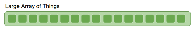
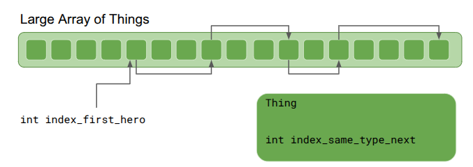
Large Array of Things
I also learned about the Large Array of Things from the Wookash podcast, in an episode with Anton Mikhailov. This data structure is basically and array of fat structs – rather than having a different collection for every entity type, you define _one_ struct that all entities, or Things, rather, use. The data structure is extremely simple – just an array of Things:
If we want lists, we can hook Things together using intrusive pointers. Any Thing can “point” to another Thing via its integer index. We get a list by maintaining an external index to the head Thing:
Iteration through the list simply starts with the first Thing and goes until the index is invalid:
int index_next = index_first_hero;
while (index_next != kInvalidThingIndex) {
   Thing& thing = things[index_next];
   DoSomething(thing);
   index_next = thing.index_same_type_next;
}
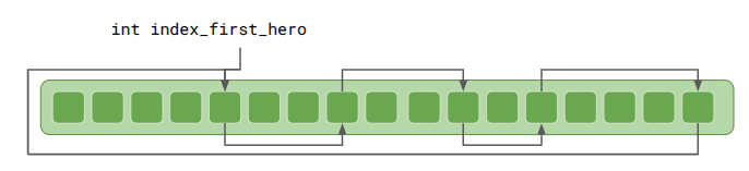
That works just fine, but we do have to (1) make sure to initialize all things with index_same_type_next = kInvalidThingIndex and (2) if we accidentally use thing.index_same_type_next with a bad index, we could go out-of-bounds. Anton recommended making all such reference lists circular:
This means thing.index_same_type_next should always be valid. If a Thing is the only one of its type, it will will point to itself.
Iteration is very similar, and has the advantage that one can start from anywhere in the list:
int index_next = index_first_hero;
do {
   Thing& thing = things[index_next];
   DoSomething(thing);
   index_next = thing.index_same_type_next;
} while (index_next != index_first_hero);
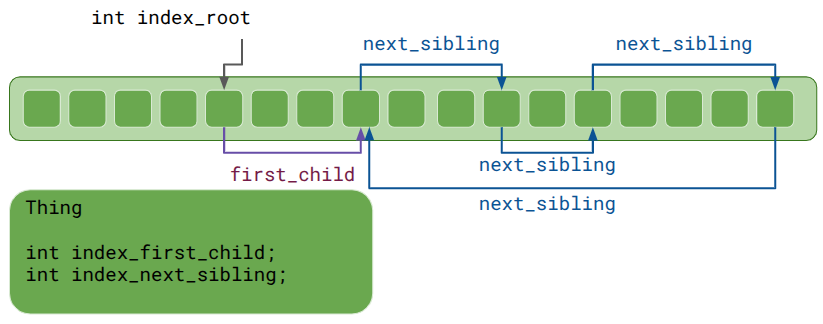
In addition to lists, indexing can also be used to represent trees:
Each Thing has a head index to a list of children, which then reference each other using sibling indices.
It makes less sense here for the head index, index_first_child, to simply point back at the same Thing, since a parent-child relationship is not a circular list. Anton Mikhailov recommended using zero for the invalid index rather than a truly invalid index like -1 in order prevent crashes. Yes, you should never access a Thing at an invalid index, but at least your game doesn’t explode in prod if a rare code path does. Plus, this means zero-initialization defaults those indices to invalid.
As a side effect, the very first Thing is never used. That is a small price to pay, especially if you’re likely going to allocate 10,000.
Lastly, Anton Mikhailov said it is often useful to use doubly-linked lists instead of singly linked lists. This makes insertion and deletion O(1). For trees, it is very useful for a child to know its parent.
So what does a Thing struct look like? Here is my current implementation:
enum class StageThingType : u8 {
    FREE         = 0, // An inactive stage thing
    HERO         = 1, // aka Player Character
    INTERACTABLE = 2,
    ROPE_SEGMENT = 3,
    COUNT        = 4, // Sentinal value
};

// A thing whose state we track in the stage.
// This follows the Large Array of Things approach.
struct StageThing {
    // The type of thing it is.
    StageThingType type;

    // The generational index of the thing in the array of things.
    ThingId id;

    // The index of the next thing of the same type.
    // This is a circular list.
    int index_same_type_next;
    int index_same_type_prev;

    // Which cell in the stage it is in.
    CellIndex cell_index;

    // The index of the next thing in the same cell.
    // This is a circular list.
    int index_same_cell_next;
    int index_same_cell_prev;

    Direction facing_dir;
    // Tree links.
    // Parents and children are always in the same cell index.
    // The sibling list is circular.
    int index_parent;
    int index_first_child;
    int index_next_sibling;
    int index_prev_sibling;

    union {
        StageThingHero hero;
        StageThingInteractable interactable;
        StageThingRopeSegment rope_segment;
    };
};
I went with a union of type-specific structures for now, since it was the most natural conversion of what I was translating from. However, team fat struct may end up convincing me. We’ll see.
We need an additional struct to store the array and the list heads:
struct LargeArrayOfStageThings {
    StageThing things[MAX_NUM_THINGS];
    int count;

    // An array of heads for doubly-linked lists.
    // Index 0 (StageThingType::FREE) is the free list.
    int type_list_heads[(int)StageThingType::COUNT];

    // An array of heads for doubly-linked lists of things in each cell.
    int cell_first_thing[GRID_MAX_X][GRID_MAX_Y];
};
As we can see, the StageThing type zero is for free / inactive Things, letting us use the same list to quickly grab the next available Thing any time we spawn a new one, or stitch it into the list if a Thing is no longer needed. Then there are a bunch of methods that maintain invariants, such as initialization, getting a Thing, attaching a child to a parent, etc.
Indices maintained by the `LargeArrayOfStageThings` itself, such as the linked type list, can be simple integers. Other indices, especially external references, shouldn’t use direct indices since the underlying Thing might be removed in the interim. (This is the same problem as keeping a pointer reference to an Entity.)
The standard mitigation, which I was already employing in my ObjectPools previously, is to use a generational index. Instead of a bare index, it is an index paired with a generation counter:
struct ThingId {
    int index;  // index in the array of things
    u32 gen;    // generation counter
}
Retrieving a Thing via such an ID simply looks at the Thing at the given index, but also checks to make sure the generation counter matches. If it does, we return it. If the Thing has been deleted, or if it has been re-used, the generation counter will have been incremented, and the counter will not match. Since we’re using a u32, there is basically zero risk of wrap around. (Though you can always use u64 if that’s a problem for you.)
Sharing Concepts
Having the shared StageThing struct means we can share concepts across all entity types. The first example is the cell index. Every StageThing can be placed in a cell. This doesn’t mean I have to use it, but so far I am. The direct result is that I can have a single codepath for PlaceInCell, which doesn’t have to have branching logic for heroes vs. ropes vs. enemies, and the LargeArrayOfStageThings can automatically update the internal list of things in each cell.
This drastically simplified my event system. Before this change, the AttachTo event required distinct code paths for every single entity type. Now, attaching is universal for all entities—it is simply a parent/child relationship.
You’ll notice that the StageThingType enum does not contain Pickup or Bucket types. I actually consolidated those into a single type – Interactable. This happened when I started considering how a Pickup could be set down or picked up, but so too could a Bucket. The Bucket simply had additional capabilities, such as allowing other things to be placed in it.
The aha moment here is recognizing that we care about functionalities rather than what a thing is categorically. So, the Interactable has a bitmask that identifies what the thing can do – can it be placed, hung, acquired, used to contain other things, etc? When it comes to the code logic, that is ultimately what it needs to know. Do I or do I not run the logic for this capability?
This is exactly the insight the fat struct folks advocate for. Seeing this simplification, I am seriously tempted to go all-in on the fat struct approach.
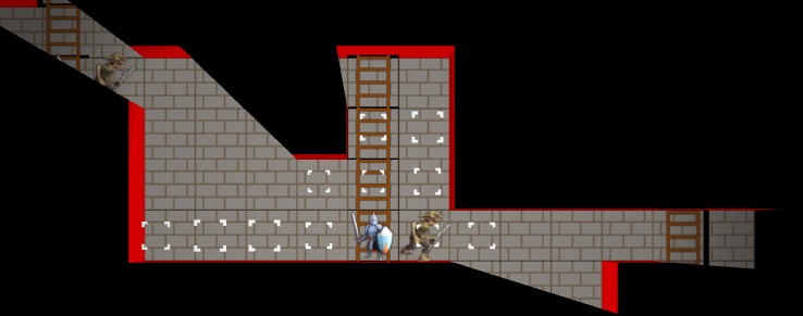
The final part of simplification was now recognizing that all entities are contained in at most a single cell. Prior to this, my rope entity spanned multiple cells. I now have a RopeSegment type instead, which is exactly one cell and has links to the RopeSegment it is connected to above or below. This works really well with the centralized cell lists and handles portals seamlessly.
Here we see a rope being lowered through a portal. The sorceress then climbs down it.
Undo and Redo
I want undo and redo to be supported from the get-go, and to “just work”. Every action must be reversible, and after being reversed, we should be able to re-commit it.
In this post, I covered the event system. Any action builds out a schedule of events that then can be played out. I supported undo and redo by collapsing the schedule into just the set of events needed to get the overall state change needed. For example, if a hero moves three times, which are three cell index change events, I could collapse that into just one cell index change event for undo / redo purposes.
Unfortunately, the logic to do this got rather involved. Any new field that I added to my entities might require a new custom event that I would then have to detect and inject. I also had several “larger” events like hoisting a rope up or down that manifested as a multitude of smaller events. Moving a rope up means adjusting all RopeSegments in the chain. I’d then have to iterate over all of those to see if there were diffs, and figure out the right events to add to the undo / redo sets to get the right result. A big headache.
Instead, I shifted from a delta-based approach to a snapshot approach. I implemented a single, special master event that lets me replace an entire StageThing. That’s it. Now, undo / redo entirely consist of these snapshot events, which overwrite the entire struct (plus the pass turn event – that isn’t in the large array of things). Executing an undo or redo simply applies these state-overwrites and then triggers a rebuild of type_list_heads and cell_first_thing in the LargeArrayOfStageThings. Incredibly simple. Since we’re not undoing and redoing all that often, the cost of that rebuild is insignificant.
Conclusion
I’m happy to have this entity refactor behind me, but I also feel like it was a great architectural experience and showed how simplicity can compound. This new foundation feels like a good one to build out from. I plan to start expanding on these core mechanics and perhaps touch up some of those rough first-pass graphics. As always, no promises on specifics! We will let the project dictate how it should evolve next.
A debug view showing shadow cast segments from the vantage point of the actor.
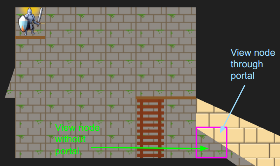
Last month we covered the unified action system, in which we built some basic things players can do with their heroes, and set the stage for fancier futures and actions for enemy agents. The most significant action was moving, which was built based on a GridView of what the actor sees from their current vantage point. As noted in that post, we eventually wanted to expand the grid view to include edge information, such as thin little walls and platforms, but also portals that act as non-Euclidean connections to other parts of the map.
Here we have a simple two-tile room with a loop-back portal on either end. The result – the hero can see a bunch of versions of themselves!
In the last post, I said I’d be adding other entities in and adding more actions, but I decided that the map representation was so fundamental that prioritizing getting these portals in was more important. Any changes there would affect most other systems, so I wanted to get that done first.
Grid Representation
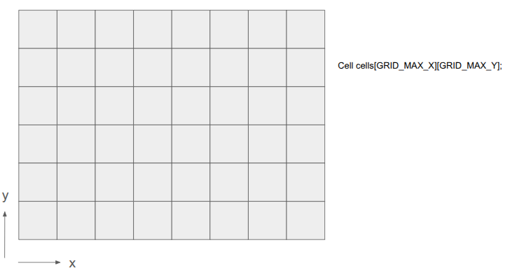
Prior to this change, the underlying level geometry representation, the Grid, was just a 2D array of cells:
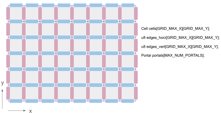
After this change, I wanted to represent both the cells as well as the edges between them:
This was achieved by adding two additional 2D arrays, one for the horizontal edges and one for the vertical edges. There are definitely other ways to do this, but I felt that (1) this was simple, and (2) there are differences between those edge types. A player might stand on a platform but have a door that they can open, for example.
The edges are single-bit entries, to keep things efficient. If we need more information, we can index into a separate array. I’m currently using the first two bits to identify the edge type, and the remaining 6 bits, if the edge is a portal, index into a Portal array. The Portal stores the information necessary to know which two edges it links.
This change has the immediate consequence that getting the cell neighbor in a given direction does not necessarily produce the Euclidean neighbor. Its second consequence is that cells no longer need to be solid or not — the edges between cells can instead be solid. This slightly simplifies cells.
Grid View Representation
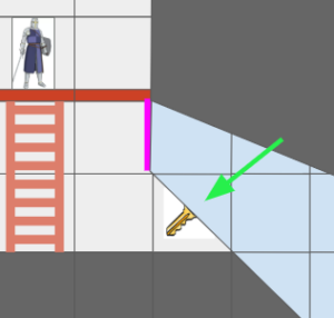
The Grid View, introduced in the last post to represent the level geometry as seen by an actor from their vantage point, can now represent views where the same underlying cell might show up multiple times due to portal connections. Furthermore, we might have weird cases where one square cell might contain slices from different areas of the map:
The green arrow points at a view cell which, due to the portal (magenta), has two sections of different grid cells.
Before, the grid view was a simple 2D array with one cell per tile. Now, that is no longer the case.
The updated grid view is organized around ViewNodes, ShadowSegments, and ViewTransforms:
struct GridView {
    // The grid tile the view is centered on
    CellIndex center;

    // The first ViewNode in each view cell.
    // 0xFFFF if there is no view node in that cell.
    u16 head_node_indices[GRID_VIEW_MAX_X][GRID_VIEW_MAX_Y];

    u16 n_nodes;
    ViewNode nodes[GRID_VIEW_MAX_NODES];

    // Shadowcast sectors.
    u16 n_shadow_segments;
    ShadowSegment shadow_segments[GRID_VIEW_MAX_NODES];

    // The transforms for the view as affected by portals.
    u8 n_view_transforms;
    ViewTransform view_transforms[GRID_VIEW_MAX_TRANSFORMS];
};
Most of the time, a given cell in the grid view will contain a single cell in the underlying grid. However, as we saw above, it might see more than one. Thus, we can look up a linked list of ViewNodes per view cell, with an intrusive index to its child (if any). Each such node knows which underlying grid cell it sees, whether it is connected in each cardinal direction to its neighbor view cells, and what sector of the view it contains:
struct ViewNode {
    CellIndex cell_index;

    // Intrusive data pointer, indexing into the GridView nodes array,
    // to the next view node at the same ViewIndex, if any.
    // 0xFFFF if there is no next view node.
    u16 next_node_index;

    // Whether this view node is continuous with the view node in the
    // given direction.
    // See direction flags.
    u8 connections;

    // The sector this view node represents.
    Sector sector;

    // The stencil id for this view node.
    // Identical to the transform_index + 1.
    u8 stencil_id;
};
We can now represent cases like the motivating portal scenario:
I’ve given the region on the other side of the portal different tile backgrounds to make it more obvious.
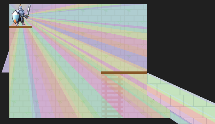
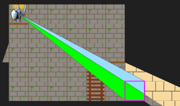
In the last post, we constructed the grid view with breadth-first search (BFS) from the center tile. Now, since we’re working with polar segments that strictly expand outwards, we can actually get away with the even simpler depth-first search (DFS). Everything is radial, and the farther out we get, the narrower our beams are:
A debug view showing the final shadow cast segments.
The search logic is a bit more complicated given that we have to narrow down the segment every time we pass through a tile’s edge, we’re saving view nodes in the new intrusive linked list structure, and edge traversals have to check for portals. Solid edges terminate and trigger the saving of a shadow segment.
Portal traversals have the added complexity of changing physically where we are in the underlying grid. If we think of the underlying grid as one big mesh, we effectively have to position the mesh differently when rendering the stuff on the other side of the portal. That information is stored in the ViewTransform, and it is also given its own stencil id.
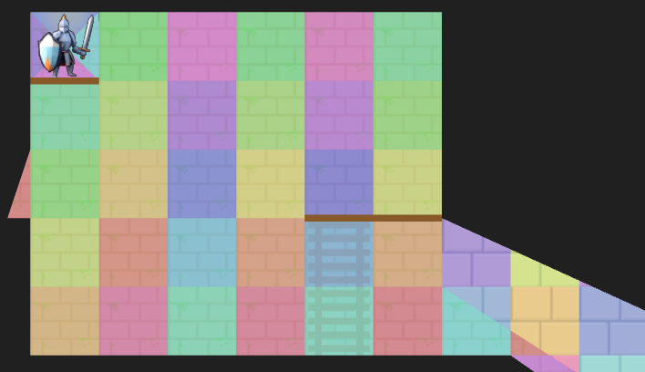
A debug view of the view nodes. We fully see many cells, but some cells we only partially see. The origin is currently split into four views in order for view segments to never exceed 180 degrees.
Above we can see an overlay of the resulting view nodes. There is a little sliver of a cell we can see for a passage off to the left, and there are the two passages, one with a portal, that we can see on the right. The platforms (little brown rectangles) do not block line of sight.
The Stencil Buffer
Now that we have the grid view, how do we render it? It is pretty easy to render a square cell, but do we now have to calculate the part of each cell that intersects with the view segment? We very much want to avoid that!
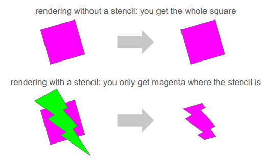
Clean rendering is accomplished via the stencil buffer, which is a feature in graphics programming that lets us mask out arbitrary parts of the screen when rendering:
We’ve already been using several buffers when rendering. We’re writing to the RGB color buffers, and 3D occlusion is handled via the depth buffer. The stencil buffer is just an additional buffer (here, one byte per pixel), that we can use to get a stenciling effect.
At one byte (8 bits) per pixel, the stencil buffer can at first glance only hold 8 overlapping stencil masks at once. However, with our 2D orthographic setup, our stencil masks never overlap. So, we can just write 255 unique values per pixel (reserving 0 for the clear).
We simply write the shadow segments to the stencil buffer, setting the buffer to the appropriate stencil ID:
The stencil buffer has four stencil masks – the red region in the main chamber, the little slice of hallway to the left, the green region through the portal leading back into the same room, and the yellow region through a different portal to an entirely different room.
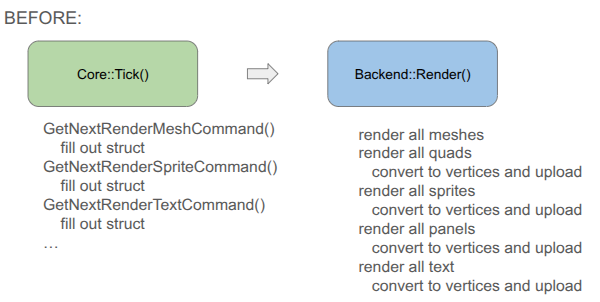
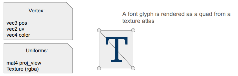
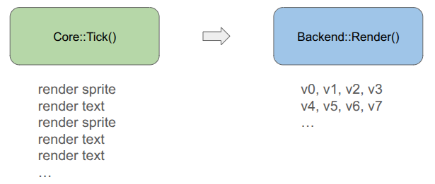
Our rendering pipeline now needs to support masking with these stencil IDs. In January we covered the render setup, which involved six different types of render commands that the game could send to the backend:
render mesh – render a 3D mesh with lighting, already uploaded to the GPU
render local mesh – render a 3D mesh without lighting, sending vertices from the CPU
render quad – an old simple command to render a quad
render sprite – self-explanatory
render spritesheet sprite – an old version of render sprite
render panel – renders a panel with 9-slice scaling by sending vertices from the CPU
render text – renders font glyphs by sending quads from the CPU
Having three versions of everything – rendering without stencils, rendering with stencils, and rendering to the stencil buffer itself, would triple the number of command types. That is too much!
Furthermore, we want to order the render commands such that opaque things are drawn front to back, and transparent things are then drawn back to front, and finally drawing UI elements in order at the end. That would require sorting across command types, which seems really messy.
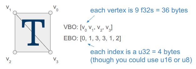
To achieve this all neatly, I collapsed everything sending vertices from the CPU to a unified command type, and have the backend fill the vertex buffer when the game creates the command:
You will notice that the game-side changed a bit. Rather than receiving a command struct and being responsible for populating all fields, I decided to move rendering to methods that expect everything you need to be passed in. This is less error prone, allows for different function signatures that populate what you need, and means I don’t actually need structs for the different command types if we’re directly converting to vertices.
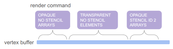
Each unified command (everything but the mesh render calls) is simply:
// Determines the order in which things are rendered.
enum class PassType : u8 {
    OPAQUE = 0,
    TRANSLUCENT = 1,
    UI = 2,
};

// Determines whether and how a command uses a stencil.
enum class StencilRequirement : u8 {
    NONE  = 0, // Does not use stencils
    WRITE = 1, // Writes to the stencil buffer
    READ  = 2, // Reads from the stencil buffer
};

// Determines how the draw gets executed.
enum class DrawMode : u8 {
    ARRAYS,   // No EBO
    ELEMENTS, // With EB
};

struct RenderCommandUnlitTriangle {
    // The commands are sorted by the sort key prior to rendering, determining the order.
    // Bits 63-62 (2 bits): Pass Type (Opaque, Translucent, UI)
    // Bits 61-60 (2 bits): Stencil Requirement
    // Bits 59    (1 bit):  Draw Mode
    // Bits 58-51 (8 bits): Stencil ID (0 for none)
    // Bits 50-32  <reserved>
    // Bits 31-0  (32 bits)
    //   In Opaque:      front-to-back distance
    //   In Translucent: back-to-front distance
    //   In UI:          sequence ID
    u64 sort_key;

    // Draw Arguments
    u32 n_vertices; // Number of vertices to draw
    u32 i_vertex;   // Index of the start vertex
    u32 n_indices;  // Number of indices, if using ELEMENTS
    u32 i_index;    // Index of the start element index, if using ELEMENTS
};
Apparently, this is much closer to how modern game engines structure their render commands. There is one vertex buffer that we write into as commands are added by the game, and the command just keeps track of the appropriate range. The same is true for the index buffer, which in our case is pre-populated buffer for quad rendering (so each quad takes 4 vertices and 6 indices instead of 6 vertices):
The pass type, stencil requirement, and draw mode are then baked into a sort key that we can sort on in order to automagically get the commands in the order we want: opaque < transparent < UI, with no stencil < write to stencil < read from stencil, and then grouping by whether we use the elements (index) buffer or not. We even use the lower 32 bits for additional sorting, rendering opaque things front to back (since lighting is expensive and we can discard more pixels that way), rendering transparent things back to front (required to get correct results), and rendering UI elements in the order they are created.
Being able to call glBufferData once to send all of the vertices up once at the beginning is really nice. Before, we were writing vertices and sending just the few we needed for every command type each time.
The end result is significantly simpler backend rendering code. It can become even simpler if we eventually unify the mesh rendering with the unlit triangle rendering, but I’m holding off on that because those render commands have a bunch of uniform data and then I’m switching between shaders. I’m not currently rendering transparent meshes, and if I eventually do I’ll bite the bullet and further consolidate.
Conclusion
I am quite happy to have tackled the fundamental grid representation, which as we saw ended up affecting a lot of stuff. The new grid view now needs to be properly integrated into the movement action, and then we can actually start introducing other entities like ropes, buckets and relics. No promises on specifics! We’ll let the project dictate how it should evolve.
Current title screen using text rendering with the Arial TrueType fonts.
Last month we covered text rendering, which was necessary for getting the scaffolding up that supports the over-arching gameplay loop. We have a title screen, a level select screen, codex screens for seeing information about unlocked heroes and relics, and a level results screen that summarizes what was gained when completing a level. All of these are rudimentary first stabs, but ya got to make it exist first.
A lot happened in the last month, some of which I might cover in future posts. I’m not going to list everything every time, but it is interesting to see just how much stuff goes into making some sort of usable interactive experience when you’re doing a lot from scratch.
Added basic hero avatars to display when the hero is selected.
Added a tweak file system for rapidly tuning parameters.
Expanded the hero struct to include a hero level state to distinguish between in-level heroes and those that have not yet been deployed and those that have exited a level.
Added new screens.
Generalized my UI panel work to have fancier button logic that properly detects button presses, accounting for when the player clicks elsewhere but releases over the button, or presses down on the button but releases elsewhere.
Moved the game interface to simply receive one large memory buffer that the game itself then chops up into whatever smaller allocations and arenas it needs.
Introduced local mesh assets that can be directly rendered via the triangle shader from the previous post, used for basic quads and things like the selection outline.
Introduced the grid view. More on that in a bit.
Added a way to quickly identify which entities are in which cells in the stage, now more necessary due to the grid view.
Introduced schedules and simulating consequences up front rather than live.
Added the action selection panel and action sub-selection interfaces for hero deployment, move selection, and turn passing. The focus of this blog post.
Removed a bunch of earlier code pre-move selection where the active hero would move one tile or perform one action per key press.
The game now looks like this:
Obviously, all art, layout, UI, etc. is an extremely early first cut and likely not the final version. We do, however, see the basic framework for a game.
Action Panel
The main thing I want to talk about this week is the fledgling action system, starting with the action panel:
The action panel shows the active hero’s avatar, their name, their level state, and has a series of action buttons.
You’ll notice that the panel has the same color as the background. Eventually, when the field of view includes shadow casting, it should just blend with the shadows. Here is my Google slides mockup of what I’m roughly working toward:
Eventually we’ll see the whole party, along with whatever status bars we need to see, and the actions available to the hero will look fancier. Most notably, I intend to render little equilateral triangles to represent the action points available for various moves. I’m not 100% settled on how that would work, but something like that will happen.
The game loop inside a level tracks which actor is active, and then loops through four states:
Generate Actions
Select Action
Play Schedule
Done
The first state is where the game looks at the current state and generates the actions available to the actor. For heroes, these then show up as options in the action panel. The user can then select an action and get access to its dedicated UI, and use that to determine the details.
Here we’ve selected the DEPLOY action and we get a user interface for selecting which cell to deploy the hero to.
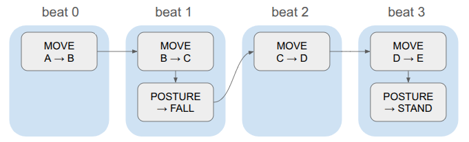
Once the user commits to an action, the action generates a schedule. This is the sequence of events that represent the outcome of the action. For example, passing the turn simply produces an event that moves the game to the next actor. Selecting a move to a cell produces a more complicated schedule that traverses multiple cells in sequence, and may involve posture changes like changing from standing to climbing.
Most importantly, a schedule contains the complete outcome of the action. Previously, if the actor planned to move, I was having the game check live, as the player moved, for triggered events like ending up over an empty shaft and then moving into a falling state. This fragments the logic and makes it harder to test planning and consequence code, as we don’t really know the consequence of an action until it is tediously simulated out over many iterations.
Instead, the schedule does all necessary consequence simulation during construction, and the game then just needs to play that out until it has completed. Given that we have the schedule, it is also quite easy to undo the entire action without having to figure out some weird reverse simulation.
This doesn’t look terribly complicated to implement, but it is actually the system that flummoxed me the most in my previous project attempt, particularly when it came to changing which actions were available based on the actor’s equipment and in enabling undo. I am much happier with how this latest rendition is set up.
The schedule is, at its core, just a DAG of events stored in a topological order:
struct Schedule {
    // Events are in a topological order
    u16 n_timeline;
    Event* timeline; // allocated on the Active linear allocator

    // The net outcome.
    u16 n_outcome;
    Event* outcomes; // allocated on the Active linear allocator

    // The opposite of the net outcome, since events are not inherently reversible.
    u16 n_undo;
    Event* undos; // allocated on the Active linear allocator
};
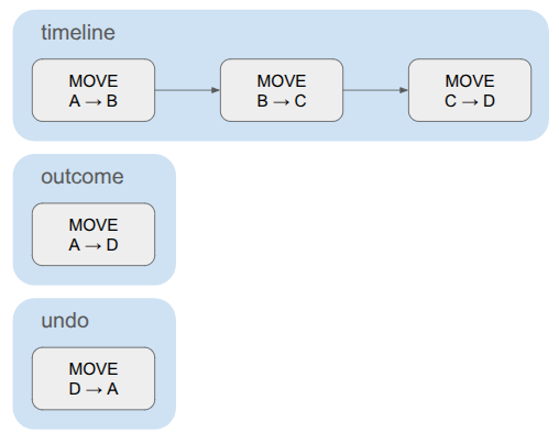
The schedule contains the full timeline, plus a compressed net outcome that only contains the events necessary to encode the overall delta. For something like a pass action, the timeline and the outcome are the same. For a move, where the actor traverses multiple cells, the timeline contains the sequence of cell traversals but the outcome only contains one cell change – from source to dest.
The schedule also contains the set of events needed to undo the action. This is very similar to the outcome, just reversed. The game events don’t all contain the information necessary to be reversed, so we construct the undo events separately.
A simple schedule for moving a hero. The timeline contains multiple cell transitions, but the outcome and undo each consist of a single event.
Events are small, composable game state deltas:
struct Event {
    u16 index;  // The event's index in the schedule. (Events are in a topological order)
    u16 beat;   // The beat that this event should be executed on. Events sharing a beat happen concurrently.
    EventType type;

    union {
        EventEndTurn end_turn;
        EventSetHeroLevelState set_hero_level_state;
        EventMove move;
        EventSetCellIndex set_cell_index;
        EventSetFacingDir set_facing_dir;
        EventSetHeroPosture set_hero_posture;
        EventAttachTo attach_to;
        EventOnBelay on_belay;
        EventOffBelay off_belay;
        EventHaulRope haul_rope;
        EventLowerRope lower_rope;
        ... etc.
    };
};
Each event knows its event type and then contains type-specific data. This is a pretty straightforward way to interleave them without annoying object-oriented inheritance code.
Events also contain beats. The game logic is discrete, and in order to have events run concurrently, we store them in the same beat:
Whenever we advance a beat, we apply all events in that beat and trigger any animations or whatnot and use that to determine how long to wait until we start the next beat. This keeps the event system clean (it doesn’t need to know how long a given animation will take, or even what animation is associated with an event), and gives us one centralized place for triggering animations and sounds.
When the schedule is fully played out, the game enters the done state and checks to see if the level is done. If not, it goes back to action generation.
The state for active levels thus includes the core game state (the stage), which actor’s turn it is, the active schedule (if any), the schedule playback state (event index, time in beat), and data for all of this turn’s actions:
struct ScreenState_Active {
    // The active playable area and the entities in it.
    Stage stage;

    // Stores data for the active actor's turn.
    Turn turn;

    // Stores the events that are scheduled to run.
    Schedule schedule;

    // The playback state of the schedule.
    PlaybackState playback_state;

    // The index of the active actor.
    int i_actor = 0;
    int i_actor_next;

    // Where we allocate the action data.
    // This allocator is only reset when actions are regenerated.
    LinearAllocator action_allocator;
};
Pretty clean when it comes down to it.
The Turn contains the actions generated for the current actor. Each action has a name, which then makes it easy to render the buttons for the actions in the action panel.
Actions
An action is a discrete state change available to an actor, such as passing the turn, moving through the environment, or attacking another actor. The available actions depend on the game state — an actor that is not yet deployed has a deploy action but no move action, and an actor with a bow should get an attack action with a ranged UI whereas an actor with a sword can only select the tiles within melee range.
To handle these things flexibly, actions have methods that can be specialized on a per-action basis. In modern C++, one would probably use objects and inheritance to implement a bunch of action subclasses. I am avoiding classes and am not using inheritance at allWhy? To see if I can, mostly. Folks like Casey Muratori hate on OOP a lot and I want to see what the fuss is., so instead we have a basic struct with some function pointers:
// A function pointer called to run the action UI for the action,
// once the action has been selected in the menu.
typedef void (*FuncRunActionUI)(GameState* game, RenderCommandBuffer* command_buffer, void* data, const AppState& app_state);

// A function pointer for a method that determines whether the action was committed.
typedef bool (*FuncIsActionCommitted)(const void* data);

// A function pointer for a method that builds a schedule from the action.
typedef bool (*FuncBuildSchedule)(GameState* game, void* data);

struct Action {
    char name[16]; // null-terminated

    // The key to press to perform this action
    char shortkey;

    // Data associated with the action, specialized per action type
    void* data;

    // Function pointers
    FuncRunActionUI run_action_ui;
    FuncIsActionCommitted is_action_committed;
    FuncBuildSchedule build_schedule;
};
We use the action name when displaying its button in the action panel, and its shortkey is available if the user doesn’t want to have to click the button with the mouse.
Each action also has a void* data member, which can be populated when the action is created and then used in the member functions. We’ll see an example of that shortly.
Generating the available actions is conceptually straightforward; just run a method for every action in the game that checks if that action is available, and if it is, allocates it, constructs it, and adds it to the action list:
This may seem too simple, but I think it is actually quite an advantage. I had previously been considering having various pieces of equipment be responsible for determining which actions they are associated with, and then having a way to store that metadata on the equipment, save it to disk, etc. Messy! Instead, I can just run all of these methods, every time, and if any require specific equipment, they can check for it and just quickly return false if it isn’t there.
Every action currently requires at least four methods: action generation, running the action-specific UI, a simple method that determines whether the user committed to the action, and a schedule generation. For the simple pass action, this doesn’t even need the void* data member:
// ------------------------------------------------------------------------------------------------
bool MaybeGenerateAction_Pass(Action* action, GameState* game, const Hero& hero) {

    strncpy(action->name, "PASS", sizeof(action->name));
    action->shortkey = 'p';
    action->run_action_ui = RunActionUI_Pass;
    action->is_action_committed = IsActionCommitted_Pass;
    action->build_schedule = BuildSchedule_Pass;

    return true;
}

// ------------------------------------------------------------------------------------------------
void RunActionUI_Pass(GameState* game, RenderCommandBuffer* command_buffer, void* data, const AppState& app_state) {
    // Nothing to do here.
}

// ------------------------------------------------------------------------------------------------
bool IsActionCommitted_Pass(const void* data) {
    return true;
}

// ------------------------------------------------------------------------------------------------
bool BuildSchedule_Pass(GameState* game, void* data) {
    ScreenState_Active& active = game->screen_state_active;

    // Build the schedule, which consists just of an end turn action.
    Schedule* schedule = &(game->screen_state_active.schedule);

    schedule->n_timeline = 1;
    schedule->timeline = (Event*)Allocate(&(active.action_allocator), sizeof(Event));
    ASSERT(schedule->timeline != nullptr, "BuildSchedule_Pass: Failed to allocate timeline!");

    CreateEventEndTurn(schedule->timeline, /*index=*/0, /*beat=*/0);

    // The outcome is the same.
    schedule->n_outcome = 1;
    schedule->outcomes = schedule->timeline;

    // The undo action: TODO

    return true;
}
The deploy action is more involved, and it does allocate a custom data struct:
struct DeployActionData {
    // List of legal entry cells for the hero.
    u16 n_entries;
    CellIndex entries[STAGE_MAX_NUM_ENTRIES];

    // The index of the entry we are looking at.
    int targeted_entry;

    // Whether the entry has been selected.
    bool entry_selected;
};

// ------------------------------------------------------------------------------------------------
void InitActionData_Deploy(DeployActionData* data) {
    data->n_entries = 0;
    data->targeted_entry = 0;
    data->entry_selected = false;
}

// ------------------------------------------------------------------------------------------------
bool MaybeGenerateAction_Deploy(Action* action, GameState* game, const Hero& hero) {

    if (hero.level_state != HERO_LEVEL_STATE_UNDEPLOYED) {
        // Hero does not need to be deployed
        return false;
    }

    ScreenState_Active& active = game->screen_state_active;
    const Stage& stage = active.stage;

    // Allocate the data for the action
    action->data = Allocate(&(active.action_allocator), sizeof(DeployActionData));
    DeployActionData* data = (DeployActionData*)action->data;
    InitActionData_Deploy(data);

    // Run through all stage entries and find the valid places to deploy
    for (u16 i_entry = 0; i_entry < stage.n_entries; i_entry++) {
        CellIndex cell_index = stage.entries[i_entry];

        ASSERT(!IsSolid(stage, cell_index), "Entry cell is solid!");

        // Ensure that the cell is not occupied by another hero
        if (IsHeroInCell(stage, cell_index)) {
            continue;
        }

        // Add the entry.
        data->entries[data->n_entries++] = cell_index;
    }

    if (data->n_entries == 0) {
        // No valid entries
        return false;
    }


    strncpy(action->name, "DEPLOY", sizeof(action->name));
    action->shortkey = 'd';
    // action.sprite_handle_icon = // TODO
    action->run_action_ui = RunActionUI_Deploy;
    action->is_action_committed = IsActionCommitted_Deploy;
    action->build_schedule = BuildSchedule_Deploy;

    return true;
}

// ------------------------------------------------------------------------------------------------
void RunActionUI_Deploy(GameState* game, RenderCommandBuffer* command_buffer, void* data, const AppState& app_state) {

    DeployActionData* action_data = (DeployActionData*)data;

    const TweakStore* tweak_store = &game->tweak_store;
    const f32 kSelectItemFlashMult = TWEAK(tweak_store, "select_item_flash_mult", 2.0f);
    const f32 kSelectItemReticuleAmplitude = TWEAK(tweak_store, "select_item_reticule_amplitude", 0.25f);
    const f32 kSelectItemFlashAlphaLo = TWEAK(tweak_store, "select_item_flash_alpha_lo", 0.1f);
    const f32 kSelectItemFlashAlphaHi = TWEAK(tweak_store, "select_item_flash_alpha_hi", 0.9f);
    const f32 kSelectItemArrowOffsetHorz = TWEAK(tweak_store, "select_item_arrow_offset_horz", 1.0f);
    const f32 kSelectItemArrowScaleLo = TWEAK(tweak_store, "select_item_arrow_scale_lo", 1.0f);
    const f32 kSelectItemArrowScaleHi = TWEAK(tweak_store, "select_item_arrow_scale_hi", 1.0f);

    // TODO: This is probably lagged by one frame.
    const glm::mat4 clip_to_world = CalcClipToWorld(command_buffer->render_setup.projection, command_buffer->render_setup.view);
    const glm::vec2 mouse_world = CalcMouseWorldPos(app_state.pos_mouse, 0.0f, clip_to_world, app_state.window_size);

    bool deploy_hero_to_target_cell = false;

    // Set the hero's location to one tile over the entry we are looking at.
    // This is a hacky way to handle the fact that the hero is not in the level yet

    // and that the camera is centered on the hero
    ScreenState_Active& active = game->screen_state_active;
    Hero* hero = active.stage.pool_hero.GetMutableAtIndex(active.i_actor);
    const CellIndex cell_index = action_data->entries[action_data->targeted_entry];
    MoveHeroToCell(&active.stage, hero, {cell_index.x, (u16)(cell_index.y + 1)});
    hero->offset = {0.0f, 0.0f};

    // Render the entrance we are currently looking at.
    {
        const f32 unitsine = UnitSine(kSelectItemFlashMult * game->t);

        RenderCommandLocalMesh& local_mesh = *GetNextLocalMeshRenderCommand(command_buffer);
        local_mesh.local_mesh_handle = game->local_mesh_id_quad;
        local_mesh.screenspace = false;
        local_mesh.model = glm::translate(glm::mat4(1.0f), glm::vec3(0.0f, -1.0f, RENDER_Z_FOREGROUND));
        local_mesh.color = kColorGold;
        local_mesh.color.a = Lerp(kSelectItemFlashAlphaLo, kSelectItemFlashAlphaHi, unitsine);

        {
            RenderCommandLocalMesh& reticule = *GetNextLocalMeshRenderCommand(command_buffer);
            reticule.local_mesh_handle = game->local_mesh_id_corner_brackets;
            reticule.screenspace = false;
            reticule.model = glm::translate(glm::mat4(1.0f), glm::vec3(0.0f, -1.0f, RENDER_Z_FOREGROUND + 0.1f));
            reticule.model = glm::scale(reticule.model, glm::vec3(unitsine * kSelectItemReticuleAmplitude + 1.0f));
            reticule.color = kColorWhite;
        }

        // Run button logic on the targeted entry.
        const Rect panel_ui_area = {
                .lo = glm::vec2(- 0.5f, - 1.5f),
                .hi = glm::vec2(+ 0.5f, - 0.5f)};
        const UiButtonState button_state = UiRunButton(&game->ui, panel_ui_area, mouse_world);

        if (button_state != UiButtonState::NORMAL) {
            local_mesh.color.x = Lerp(local_mesh.color.x, kColorWhite.x, unitsine);
            local_mesh.color.y = Lerp(local_mesh.color.y, kColorWhite.y, unitsine);
            local_mesh.color.z = Lerp(local_mesh.color.z, kColorWhite.z, unitsine);
        }

        if (button_state == UiButtonState::TRIGGERED) {
            deploy_hero_to_target_cell = true;
        }
    }

    bool pressed_left = IsNewlyPressed(app_state.keyboard, 'a');
    bool pressed_right = IsNewlyPressed(app_state.keyboard, 'd');

    // Render two arrow-like triangles that let us switch between options.
    {
        const f32 unitsine = UnitSine(game->t);
        const f32 scale = Lerp(kSelectItemArrowScaleLo, kSelectItemArrowScaleHi, unitsine);

        const glm::vec2 halfdims = glm::vec2(0.433f * scale, 0.5f * scale); // NOTE: Rotated

        { // Left triangle
            const glm::vec2 pos = glm::vec2(-kSelectItemArrowOffsetHorz, -1.0f);

            const Rect panel_ui_area = {
                    .lo = pos - halfdims,
                    .hi = pos + halfdims};
            const UiButtonState button_state = UiRunButton(&game->ui, panel_ui_area, mouse_world);

            RenderCommandLocalMesh& local_mesh = *GetNextLocalMeshRenderCommand(command_buffer);
            local_mesh.local_mesh_handle = game->local_mesh_id_triangle;
            local_mesh.screenspace = false;
            local_mesh.model =
            glm::scale(
                glm::rotate(
                    glm::translate(glm::mat4(1.0f), glm::vec3(pos.x, pos.y, RENDER_Z_FOREGROUND)),
                    glm::radians(90.0f),
                    glm::vec3(0.0f, 0.0f, 1.0f)
                ),
                glm::vec3(scale, scale, 1.0f)
            );
            local_mesh.color = kColorGold;

            if (button_state != UiButtonState::NORMAL) {
                local_mesh.color = glm::mix(local_mesh.color, kColorWhite, unitsine);
            }

            // Check for pressing the button.
            if (button_state == UiButtonState::TRIGGERED) {
                pressed_left = true;
            }
        }
        { // Right triangle
            const glm::vec2 pos = glm::vec2(kSelectItemArrowOffsetHorz, -1.0f);

            const Rect panel_ui_area = {
                    .lo = pos - halfdims,
                    .hi = pos + halfdims};
            const UiButtonState button_state = UiRunButton(&game->ui, panel_ui_area, mouse_world);

            RenderCommandLocalMesh& local_mesh = *GetNextLocalMeshRenderCommand(command_buffer);
            local_mesh.local_mesh_handle = game->local_mesh_id_triangle;
            local_mesh.screenspace = false;
            local_mesh.model =
            glm::scale(
                glm::rotate(
                    glm::translate(glm::mat4(1.0f), glm::vec3(pos.x, pos.y, RENDER_Z_FOREGROUND)),
                    glm::radians(-90.0f),
                    glm::vec3(0.0f, 0.0f, 1.0f)
                ),
                glm::vec3(scale, scale, 1.0f)
            );
            local_mesh.color = kColorGold;

            if (button_state != UiButtonState::NORMAL) {
                local_mesh.color = glm::mix(local_mesh.color, kColorWhite, unitsine);
            }

            // Check for pressing the button.
            if (button_state == UiButtonState::TRIGGERED) {
                pressed_right = true;
            }
        }
    }


    // Process the presses, which can come from keys or clicking the arrows.
    if (pressed_left) {
        CircularDecrement(action_data->targeted_entry, (int)action_data->n_entries);
    } else if (pressed_right) {
        CircularIncrement(action_data->targeted_entry, (int)action_data->n_entries);
    }

    if (deploy_hero_to_target_cell) {
        action_data->entry_selected = true;
    }
}

// ------------------------------------------------------------------------------------------------
bool IsActionCommitted_Deploy(const void* data) {
    const DeployActionData* action_data = (DeployActionData*)data;
    return action_data->entry_selected;
}

// ------------------------------------------------------------------------------------------------
bool BuildSchedule_Deploy(GameState* game, void* data) {
    ScreenState_Active& active = game->screen_state_active;

    const Hero* hero = active.stage.pool_hero.GetAtIndex(active.i_actor);
    const CellIndex src = hero->cell_index;
    const CellIndex dst = {src.x, (u16)(src.y - 1)};

    // Build the schedule, which changes the hero's level state and moves them to the entry (1 cell down).
    Schedule* schedule = &(game->screen_state_active.schedule);

    {
        schedule->n_timeline = 2;
        schedule->timeline = (Event*)Allocate(&(active.action_allocator), schedule->n_timeline * sizeof(Event));
        ASSERT(schedule->timeline != nullptr, "BuildSchedule_Deploy: Failed to allocate timeline!");

        CreateEventSetHeroLevelState(schedule->timeline, /*index=*/0, /*beat=*/0, hero->id, HERO_LEVEL_STATE_IN_LEVEL);
        CreateEventMove(schedule->timeline + 1, /*index=*/1, /*beat=*/0, hero->id, Direction::DOWN, src, dst);
    }

    // The outcome is the same.
    schedule->n_outcome = 1;
    schedule->outcomes = schedule->timeline;

    // Undo: TODO

    return true;
}
Move Actions
The move action is significantly more complicated than the deploy or pass actions.
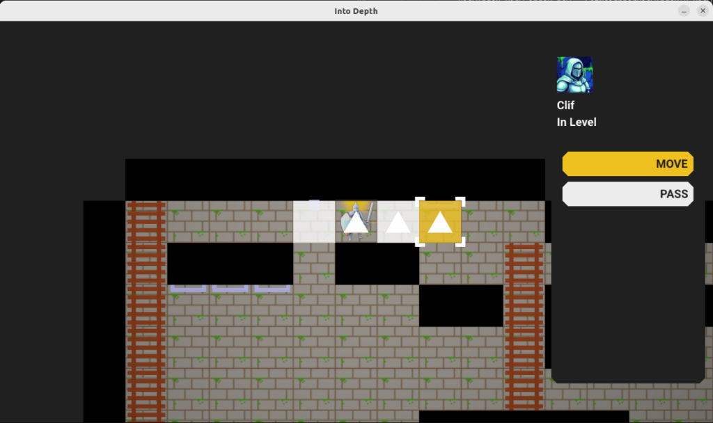
The move action highlights all valid target cells, allowing the player to select one to move to. Once selected, the shortest path to that cell is taken by the hero, and all consequences are simulated (e.g. falling, triggering a trap) and built into a schedule.
The move action UI, which here has three valid target cells (since falling ends the search). The tile under the mouse cursor is highlighted in yellow, has square angle brackets, and the shortest path is shown as a trail of equilateral triangles.
In order to support these features, the move action logic needs to know what the reachable cells are and what the shortest paths to them are. This is achieved by running Dijkstra’s algorithm from the actor’s initial state. The state space is not merely cell positions, but also includes the actor’s facing direction and their posture (standing, on ladder, etc.).
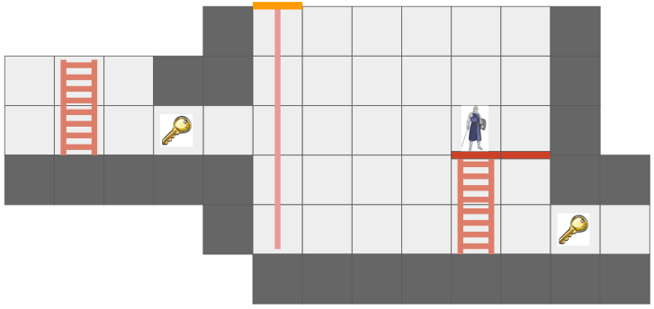
There is one additional point of complication, and that is that we want this game to only reason about cells that are visible from the hero’s current vantage point, and we eventually want to support non-Euclidean connections like portals:
In this mockup, the key is visible twice because the hallway has a portal loop-back connection.
In order to achieve this, we introduce a new representation of the level geometry visible to an actor, the GridView:
struct GridView {
    // The grid tile the view is centered on
    CellIndex center;

    CellIndex cell_indices[GRID_VIEW_MAX_X][GRID_VIEW_MAX_Y];
    u8 flags[GRID_VIEW_MAX_X][GRID_VIEW_MAX_Y];
};
This view has a finite size, much smaller than the overall level grid, that is big enough to fit the screen. The view is always centered on an actor, and the cells in the view are then indices into the cells in the underlying level grid. If a level grid cell is connected by a non-Euclidean portal to another cell, the view can just index into the correct cells on either side of the portal. Constructing the grid view is a straightforward breadth-first search from the center tile.
Note: I am actually temporarily making this simpler than it really is. To do this properly, we’ll need a fancier data structure that is not a grid but can handle sectors, because one view cell may actually contain view sectors of multiple level cells:
This view cell is visible twice, once with a cell containing a key, with this portal (magenta) set up.
We thus run Dijkstra’s algorithm in this grid view, starting from the center cell where the actor is. The same cell may be visible multiple times in the grid view, and we will correctly be able to route to that cell via multiple paths.
The search assigns a cost for each state change, and only searches up to a maximum cost. Very soon, actors will have action points to spend per turn, and it won’t be possible to move further than are affordable given the action points currently available.
The move action custom data struct is:
struct MoveActionData {
    // We can only ever move to a visible tile, so for now, we can
    // just allocate a grid's worth of potential targets.

    // The cheapest cost to reach each move state.
    u16 costs[GRID_VIEW_MAX_X][GRID_VIEW_MAX_Y][/*num directions=*/2][kNumHeroPostures];

    // The parent state on the shortest path that arrives at the given state.
    // I.E., if [1][2][LEFT][STANDING] contains {2,2,LEFT,STANDING}, then we took a step over.
    // The root state points to itself.
    MoveState parents[GRID_VIEW_MAX_X][GRID_VIEW_MAX_Y][/*num directions=*/2][kNumHeroPostures];

    // Used to track whether a view cell has been visited.
    u32 visit_frame;
    u32 visits[GRID_VIEW_MAX_X][GRID_VIEW_MAX_Y];

    ViewIndex view_index_target;  // Target view cell index for the move.
    bool entry_selected;
};
Having completed the search, we are able to render all reachable tiles, render a reticle over the cell the user’s mouse is over, and if the cell is reachable, we can backtrack over the cell’s parents to render the cells traversed to get there. (Since states include more than just cell changes, and we don’t want to render multiple times to the same cell, we also store a u32 visit frame that we can use to mark cells we have rendered to in order to avoid rendering to the same cell multiple times.)
Finally, when the user clicks on a cell to commit the action, we compute the schedule by:
Extracting the shortest path by traversing back to the source node.
Writing the shortest path out one state change at a time.
Simulating consequences (like falling) after every step, and if any consequences do take place, ending the planned schedule there and appending all consequence events.
This process makes a copy of the current state and applies all changes there. Making a copy, while taking memory, has the advantage of not polluting the actual game state and giving us a second Stage to compare the current Stage to in order to get the overall schedule delta.
Conclusion
With the action system in place, the foundation is laid for actual gameplay. Next time, we’ll look at introducing some core entities back in (ropes, buckets, relics) and managing the overall gameplay cycle.
Into Depth is the name of a little game project I have been working on for over a year now. Its roots go back even further, to the 2D platformer I had started working on two years ago. The platformer ended up teaching me a lot about OpenGL, which I have continued to use in a fairly low-level manner in this new project.
Concept image by ChatGPT.
In a nutshell, the game is a simplification of the 2D platformer born both from managing complexity and wanting something I could reasonably make multiplayer and play with my friends online. Into Depth is a turn-based 2D sidescroller on a grid. Kind of like Gloomhaven, but vertical:
An early mockup from my Google slides design doc.
The team of heroes descends into dungeons (e.g., down the rope in the image above) with the goal of retrieving relics. Oftentimes these relics are heavy and require hauling to get them back to the surface. Collected relics can be equipped and used in other levels, and teams may revisit levels in order to get even deeper. That’s the rough idea.
There are additional details, of course. For example, I want non-Euclidean geometry to play a role. In the screen above, the two edges labeled ‘a’ are joined, such that the hero’s view is:
The hero can see the key from two different vantage directions because of the portal.
This is made more interesting by having each hero only be able to see what is in their line of sight. Not only does that add an element of discovery and the need to juggle teammates’ perspectives, it also enables stealth mechanics.
Solid geometry blocks the view of what is behind it. This image was from before I went orthographic.
I am writing this myself, for fun, in my spare time. My primary goal is to learn how things work, and to actually get something playable for myself and my friends.
Why these restrictions? Because I am a big fan of Casey Muratori, Jonathan Blow, and the do-it-yourself attitude of understanding your code. It is a great way to learn how it all works, and it is fun! Presumably it leads to smaller executables and faster code too.
The art you see here is programmer art, since I am a programmer. That is good enough for now. My long-term vision is to have a low-poly aesthetic and mostly not use sprites, since I should be able to author low-poly meshes myself. The scene will be 3D with effects like lighting, but will be rendered in orthographic since that just makes it so much easier to see and work with the grid.
Font Glyphs + Sprites
I was most recently working on some basic shaders for the game. I had just added font rendering with its own shader for rendering glyph quads. A UI system typically needs things beyond just font glyphs, like UI panels and sprite icons, and those are mostly just basic quads as well. It seemed obvious that I could share a shader for the dual uses of rendering font quads and rendering sprite quads:
The shader is really simple. In the vertex shader, the position is just:
gl_Position = proj_view * vec4(aPosWorld, 1.0);
And then the fragment shader uses the input color as a componentwise multiplier after looking up the texture value via the UV coordinate:
vec4 tex_color = texture(u_texture, uv);
FragColor = color * texture_rgba;
The font atlas has white glyphs, which means this color multiplier produces fonts that look like we want. Colored sprites are typically rendered with color = [1,1,1,1] so that we don’t affect them, but you can also tint them by changing up the values.
Rendering quads is also straightforward, but when you’re doing it all yourself, there is still a fair amount of stuff to keep track of. Every glyph in the font has a packed quad that tells us its size and its UV coordinates in the font atlas. We write the quad vertices into a VBO, and rather than writing six vertices to get the two triangles per quad, we only write the four unique ones and use an EBO to define the quads by indexing into the vertex array (as is standard practice):
Each frame, the backend fills up a vertex buffer and sends it to the VBO for rendering. This only needs to happen once, if the sprites and the font glyphs are all packed into the same texture and everything uses the same projection and view matrix.
Render Commands
The core game code does not directly fill the vertex buffer. Instead the core game code issues more simple render commands. These commands are simple, higher-level descriptions of what we want rendered, making the core game code fast and separating out the task of deciding how to render everything up to the backend.
For example, a render text command is:
struct RenderCommandTextLine {
    FontHandle font_handle;
    glm::vec2 pos;       // Bottom-left of the first glyph
    f32 letter_size;     // Multiplier off of default
    f32 letter_spacing;  // Multiplier off of default
    s8 text;             // Must last until rendered
    glm::vec4 color;     // RGBA componentwise color multipliers
};
It is up to the backend to convert that higher-level specification into the actual quad vertices, moving that non-trivial logic out of the core game loop and into its own location. The render command thus acts as an API between the game and the backend. Any new backend that we support in the future must be able to render these things.
In the future, when I might have partially transparent objects, the backend can do more sophisticated things like render all opaque geometry first and then sort the transparent objects by depth and render them in a second pass. Something like that is very hard to do when the core logic is rendering as it goes.
Including Triangles
So far, we have a shader that can render both font glyphs and sprites. That’s nice, but I want Into Depth to have a low-poly, flat-color aesthetic. I wanted to add UI panels that underlay the text, and I want those to be tessellated:
A panel like that is comprised of a relatively small number of triangles when compared to a modern 3D character mesh (~40 vs. 1000’s). It should be cheap enough for us to directly write that geometry out every frame.
Our font + sprite shader can actually be used to draw basic triangles, we just need to point all three vertices of the triangle to all-white uv coordinates so that we get the color we want. This is achieved by including a \(1 \times 1\) white spriteThis technique was mentioned in the Wookash Podcast with Omar Cornut of Dear ImGui..
I thus define some additional render commands, such as RenderCommandPanel, that act as high-level descriptions of what should be rendered, and then have the backend construct the mesh live in the vertex buffer and send it over. Doing this does not use the quad-specific EBO, so for now I’m just using a glDrawArrays call instead of a glDrawElements call.
I did make one adjustment to the shader – rather than switching out the textures depending on my use, I just have an array of textures that I can leave bound and have each vertex declare which one its UV coordinate applies to:
I pack my fonts into a font atlas that is uploaded as the first texture, then have a series of sprite atlases.
Sprite Packing
I need to bake my font glyphs and my sprites into a series of textures that my shader can then use. There are plenty of tools that do sprite packing for you. I was already using stb_truetype and stb_rect_pack to create my font atlas, so I decided to write my own sprite packer on top of stb_rect_pack.
Conceptually, it is really simple. I give it a set of individual sprites, and it keeps trying to pack as many as possible into a new texture until everything is packed. The only little gotcha is that a \(w \times h\) sprite is packed as a \(w+2 \times h+2\) rectangle in order for it to be padded with a 1-pixel extended border to fight edge bleeding caused by inaccuracies in UV coordinates between mipmap levels.
Shader Code Organization
Beyond assets, shaders themselves tend to more complexity than you’d think because the code to use them ends up spread all over the codebase. The vertex and fragment shader definitions are often two separate .glsl files, which live in their own folder alongside the other shaders. The C++ side typically needs a vertex struct defined somewhere, and then we need both CPU-side vertex buffers and references to the GPU-side shader program IDs, VAO, VBO, and EBOs. Whenever we use a shader, we need to activate it, which involves more code that has to use these references and set various shader uniforms.
I’ve adopted a few enhancements to reduce the degree of code spread.
The first thing I did was unify the vertex and fragment shaders into a single .glsl file. Since we just read in the file and upload it to the GPU before calling glCompileShader, we can actually process out the necessary portions ourselves. Writing both shaders in the same file helps keep their interdependencies consistent.
#version 330 core
#ifdef VERTEX_SHADER
layout (location = 0) in vec3 aPosWorld; layout (location = 1) in vec4 aVertexColor; // rgba layout (location = 2) in vec2 aTexCoords;
This was nice, but I actually ended up further simplifying by having a single .h file that defines the shader data relevant to the CPU side. The vertex and fragment shaders are still defined in one place, but as explicit strings, and we additionally define a vertex layout:
#pragma once

#include "util/strings.h"
#include "util/vertex_layout.h"

constexpr int kNumUnlitTriangleShaderTextures = 8;

// The vertex data structure (CPU-side)
struct UnlitTriangleVertex {
    glm::vec3 pos;
    glm::vec4 rgba;
    glm::vec2 uv;
    int texture_index;
};

// The shader definition
struct UnlitTriangleShaderDefinition {
    static constexpr const char* kName = "UnlitTriangle";

    static constexpr VertexElement kVertexElements[4] = {
        {ShaderDataType::Vec3F, "aPosWorld", false, offsetof(UnlitTriangleVertex, pos          )},
        {ShaderDataType::Vec4F, "aRGBA",     false, offsetof(UnlitTriangleVertex, rgba         )},
        {ShaderDataType::Vec2F, "aUV",       false, offsetof(UnlitTriangleVertex, uv           )},
        {ShaderDataType::I32,   "aTexIndex", false, offsetof(UnlitTriangleVertex, texture_index)},
    };

    static constexpr VertexLayout kVertexLayout = {
        kVertexElements,
        sizeof(kVertexElements) / sizeof(kVertexElements[0]),
        sizeof(UnlitTriangleVertex)
    };

    static constexpr const char* kVertexShaderSource = R"(
        #version 330 core

        layout (location = 0) in vec3 aPosWorld;
        layout (location = 1) in vec4 aRGBA;
        layout (location = 2) in vec2 aUV;
        layout (location = 3) in int  aTexIndex;

             out vec4 rgba;
             out vec2 uv;
        flat out int  texture_index; // 'flat' means do not interpolate

        uniform mat4 proj_view; // proj * view

        void main()
        {
            gl_Position = proj_view * vec4(aPosWorld, 1.0);
            rgba = aRGBA;
            uv = aUV;
            texture_index = aTexIndex;
        }
    )";

    static constexpr const char* kFragmentShaderSource = R"(
        #version 330 core

             in vec4 rgba;
             in vec2 uv;
        flat in int  texture_index;

        out vec4 FragColor;

        uniform sampler2D textures[8];

        void main()
        {
            vec4 texture_rgba;

            // The 'switch trick' is faster/safer on some drivers.
            switch(texture_index) {
                case 0:  texture_rgba = texture(textures[0], uv); break;
                case 1:  texture_rgba = texture(textures[1], uv); break;
                case 2:  texture_rgba = texture(textures[2], uv); break;
                case 3:  texture_rgba = texture(textures[3], uv); break;
                case 4:  texture_rgba = texture(textures[4], uv); break;
                case 5:  texture_rgba = texture(textures[5], uv); break;
                case 6:  texture_rgba = texture(textures[6], uv); break;
                case 7:  texture_rgba = texture(textures[7], uv); break;
                default: texture_rgba = vec4(1.0,0.0,1.0,1.0); break; // magenta
            }

            FragColor = rgba * texture_rgba;
        }
    )";
};
The vertex layout is just a programmatic representation of the inputs to the Vertex shader. This avoids having to have VBO-creation code that lives elsewhere depend on this shader. We can go from code like this:
My OpenGL backend has the general SetUpVertexAttrib, but it doesn’t have to change if we change the shader. The backend additionally has structs for the GPU object references, the shader uniforms, and their locations:
struct UnlitTriangleShaderRefs {
    GLuint shader_program_id;

    GLuint vao; // vertex array object
    GLuint vbo; // vertex buffer object
    size_t vbo_tri_capacity;  // Number of triangles we have space for in the VBO.

    GLuint ebo_quads; // prepopulated with quad indices
};

struct UnlitTriangleShaderUniforms {
    GLint uniformloc_proj_view; // proj * view from glGetUniformLocation
    GLint uniformloc_textures;

    GLuint texture_ids[kNumUnlitTriangleShaderTextures];
};
This organization scheme has, so far, been much nicer to work with.
Conclusion
When you are writing everything yourself, there is a lot to keep track of. Most of my previous attempts at coding a game “from scratch” struggled under mounting complexity. Unifying font, sprite, and basic unlit geometry rendering under one shader helps alleviate that complexity. Even more so, having good separations of concern between the core game logic and the backend lets the game logic just have simple references to assets and focus on the game, and the backend figure out how to fill vertex buffers and ship them to the GPU.
Early in 2025, I had stumbled on concept images of a font with triangular glyphs. Something about it was appealing. I ended up crafting a similar concept, but extending it so that the equilateral triangles could tile together using both upward and downward facing triangles:
The upward and downward facing glyphs for the triangle font, from A to Z.
I was implementing OpenGL font rendering in C++, using Sean Barrett’s TrueType library to load fonts and construct a font atlas. Somewhere in this whole process I decided it would be fun to implement a font I had conceptualized months ago for real, so to speak, as a TrueType font.
TrueType doesn’t support conditional logic for alternating glyph directions like this, so in practice I achieve the effect by making all uppercase characters be upward facing triangles and all lowercase characters be downward facing triangles. The text below is “HeLlO wOrLd”:
HeLlO wOrLd
Having my own game that could load and use the font was helpful for debugging, once the binary was loadable, since I could step through it with a debugger. I also found fontdrop and the hex editor useful.
There are two fundamental responsibilites: defining the font in memory and serializing it to .ttf:
FontDefinition font = CreateFont();
bool success = ExportFont(&font);
Separating font definition from binary export keeps the system reusable and avoids hard-coded constants leaking into the writer.
CreateFont populates a builder struct:
FontDefinition font;
assert(InitFontDefinition(&font,
    /*units_per_em=*/1000, /*ascent=*/866,
    /*descent=*/0, /*line_gap=*/0,
    /*family_name=*/"TeSsElLaTe",
    /*subfamily_name=*/"Regular",
    /*unique_name=*/"TeSsElLaTe rEgUlAr v1.0",
    /*full_name=*/"TeSsElLaTe rEgUlAr")
  && "Failed to initialize font");

// Create the missing glyph (.notdef) - a simple square
// This glyph is shown when a character is not found in the font
const GlyphId missing_glyph = StartGlyph(&font, /*codepoint=*/0, advance_width, left_side_bearing);
assert(missing_glyph != 0xFFFF && "Failed to start missing glyph");

// Create a square contour with 4 points
assert(StartContour(&font) && "Failed to start contour for missing glyph");
assert(AddPoint(&font, 0, 0, 1) && "Failed to add point 0");
assert(AddPoint(&font, 1000, 0, 1) && "Failed to add point 1");
assert(AddPoint(&font, 1000, 1000, 1) && "Failed to add point 2");
assert(AddPoint(&font, 0, 1000, 1) && "Failed to add point 3");
assert(EndContour(&font) && "Failed to end contour for missing glyph");
assert(EndGlyph(&font) && "Failed to end missing glyph");
The font definition is kept in a truetype.hpp header, along with builder helpers like StartContour and AddPoint. After defining all of the glyphs, we can also add kerning pairs. The default xadvance is set for subsequent equilateral triangles, and I reduce that for pairs that nest together.
ExportFont needs to open a file and write the binary .ttf file. The format consists of a directory listing the tables and their offsets, followed by the tables themselves, padded to 4-bytes. Each table has a checksum, and the data is exported as big-endian (not the default when using fwrite).
I wanted to calculate the table checksums as I wrote to disk to avoid multiple passes over the data. This requirement was realized via a TableWriter struct along with some basic helper methods like WriteU16BE(&writer, value), which exports the value in big-endian and updates the checksum.
All WriteXXBE helper methods call down to a void FeedBytesToChecksum(TableWriter* writer, const u8* data, u32 size); method, which appropriately updates the checksum and writes the data to the file.
After writing placeholder values for the directory, the exporter writes all of the tables, in alphabetical order. Each table is written as follows:
Offset values are captured directly from the file stream as each table is written to disk, enabling a single streaming pass without rewinding or recomputing. Each table has its own WriteXXXXTable method, all of which were kept in a truetype_export.hpp header. This made it easy to iterate on the code.
We then go back and update the table directory. Easy peasy.
Finishing a Vertical Slice
I didn’t know whether the font exporter was working until I was able to load the resulting .ttf file in another program. A vertical slice lets you de-risk binary exporters early. I prioritized this by not immediately defining all glyphs and instead just defined the undefined glyph (.notdef), space, and ‘A’. I implemented the minimum necessary set of TrueType tables that could be loaded by tools like stb_truetype and the browser inspector, helping me confirm correctness before scaling out to A–Z and a-z.
Having a testable vertical slice is essential when coding on any project, whether solo or on a team. Coding without knowing whether your code is working is the same as flying blind. A hex editor provides directional confidence that the structure is forming correctly, but real validation only comes when another program successfully loads the font.
Bugs
Sometimes it is interesting to look at what sorts of issues you run into. Understanding how a process fails tells you where to focus on improvements. The bugs that I spent time investigating were:
Glyph alignment (segfault). Each glyph must be word-aligned. IMO, this is not at all obvious from the glyf table documentation.
Malformed contours as a result of exporting glyph vertices rather than relative vertices. This was clearly laid out in the documentation.
Lastly, kerning was working in my font rendering but not for all characters in chrome. It turned out that almost all of my glyphs start at (0,0), but a few, like ‘d’, did not. Chrome was rendering these further to the left. I had to set the left side bearing for those glyphs.
So two counts of failing to use alignment. Seems like a trend I can be more aware of. Despite chasing binary alignment and metrics, I ran into no memory safety issues like null pointers or leaks — problems typically cited as risks of low-level code.
Initializer Lists
I am trying to write in a Muratori-inspired minimal C++ style. That is, C++ without a lot of the C++ features. Avoid classes, macros, templates, and the standard libraries. Why? Ostensibly because simpler code is sufficient, and then easier to understand and faster to compile / execute. Though doing it because I think it is interesting and I admire people like Casey and attitudes like this one from Chris Wellons is also a perfectly valid reason.
I was able to author everything to adhere to this style, but found that I really did want to use initializer lists to simplify glyph creation:
assert(AddGlyph(&font, 'A', advance_width, left_side_bearing,
        {{A, D, N, O, E, B, C}, {S, L, R}}) && "Failed to add A glyph");
assert(StartContour(&font) && "Failed to start contour"); assert(AddPoint(&font, font.units_per_em*A.x, font.units_per_em*A.y, 1) && "Failed to add point"); assert(AddPoint(&font, font.units_per_em*D.x, font.units_per_em*D.y, 1) && "Failed to add point"); assert(AddPoint(&font, font.units_per_em*N.x, font.units_per_em*N.y, 1) && "Failed to add point"); assert(AddPoint(&font, font.units_per_em*O.x, font.units_per_em*O.y, 1) && "Failed to add point"); assert(AddPoint(&font, font.units_per_em*E.x, font.units_per_em*E.y, 1) && "Failed to add point"); assert(AddPoint(&font, font.units_per_em*B.x, font.units_per_em*B.y, 1) && "Failed to add point"); assert(AddPoint(&font, font.units_per_em*C.x, font.units_per_em*C.y, 1) && "Failed to add point"); assert(EndContour(&font) && "Failed to end contour");
assert(StartContour(&font) && "Failed to start contour"); assert(AddPoint(&font, font.units_per_em*S.x, font.units_per_em*S.y, 1) && "Failed to add point"); assert(AddPoint(&font, font.units_per_em*L.x, font.units_per_em*L.y, 1) && "Failed to add point"); assert(AddPoint(&font, font.units_per_em*R.x, font.units_per_em*R.y, 1) && "Failed to add point"); assert(EndContour(&font) && "Failed to end contour");
assert(EndGlyph(&font) && "Failed to end glyph");
You can see why I wanted to save myself the typing.
Unfortunately, in addition to including <initializer_list>, I also ended up including <vector> because I was calling AddGlyph with a transform for all downward facing glyphs:
assert(AddGlyph(&font, 'f', advance_width, left_side_bearing,
        ReflectToDownwardGlyph({{A,B,F,J,N,U,V,S,G,C}}, t))
        && "Failed to add f glyph");
Unfortunately, I couldn’t have ReflectToDownwardGlyph modify an initializer list and produce a new one. Instead, I had to return an std::vector. Oh well.
There probably are reasonable ways to do this in an minimal style. If you happen to know, please send me a message!
Conclusion
It was fun to work on a self-contained, somewhat artistic project. I got a chance to try both the Cursor and Antigravity agentic IDEs, both of which worked quite well.
I’m not sure that I’ll be able to author posts monthly, but hopefully this is a good start to returning to my creative outlet. Happy Holidays!
When I was first learning about deep learning, the teacherI think it was Andrej Karpathy teaching CS 231n. brought up an issue with image classifiers and black swans. I would call this the black swan problem, but it turns out that has a related but different meaning, so let’s go with swan classifier generalization problem. It goes like this:
If you train a classifier to identify objects in images, and one of those categories is swans, that classifier will tend to be training exclusively or predominantly on white swans. At deployment it is likely to misclassify images of Australian black swans.
This isn’t all that surprising. Generalization in deep learning is hard.
What is surprising is:
Most humans familiar with swans would be able to recognize an Australian black swan as a swan.
In other words, humans are good at generalization and are able to do it better than many of our traditional deep learning tools, at least in comparison to ImageNet and other, older, deep image classifiers.
This post is an exploration into deep learning, classification, and generalization, and about why I think feature embeddings go a long way to building a better knowledge representation. None of this is particularly new or insightful – I just find it useful to work it out and tie it all together.
Grandmother Cells
A deep image classifier takes as input an image and produces as output a softmax distribution over a discrete set of categories:
Conventional knowledge is that deeper levels reason about more sophisticated, higher-level features. Very early convolutional layers typically only have access to small neighborhoods of pixels, so learn local features like edge detections and textures. Deeper layers might piece together larger structures like a bird beak or ripples in a lake. Finally, all of this information is brought together to produce the final classification.
Under such an approach, you literally have one, single neuron at the end responsible for firing when it thinks the image has a swan. The more intensely its output value, the more confident the swan prediction.
There have historically been two opposing views on the relationship between brains and behavior — the localistview that specific brain regions are responsible for specific behaviors, and the holistic view that neural activity is spread out throughout the nervous system. A critic of the localist view might think it absurd that there is a single neuron somewhere in your head that fires over the concept of “Grandmother”.
A grandmother cell is just that — a neuron exclusively dedicated to one high-level but specific concept. (Funny enough, there was a lot of hubbub in 2005 about recordings that suggested that a single neuron had been found that triggers only for Jennifer Aniston.)
By and large, researchers do not believe that the best way to represent knowledge is through a 1:1 representation such as grandmother cells. As such, it may not come as a surprise when a traditional convolutional deep image classifier like ImageNet struggles to classify black swans.
Sparse Encodings
A traditional image classifier is structured to prefer sparse outputs. A confident prediction should produce a high value in the appropriate category and very low values elsewhere:
If the model is uncertain, it is forced to make the appropriate trade-off to assigning some probability mass to the other potential categories. That might mean assigning some likelihood to other black birds:
This sort of representation might be convenient for the output of a classifier, but it isn’t all that useful for reasoning. If I am trying to think about what it means for an object to be a swan, I don’t want to simply know it is a swan, I want to think about where I might find it (e.g. on a lake), what it might do (e.g. honk at me), and sure, what it looks like (e.g. tends to be white-feathered).
A reasoning network that receives the fact that there is a swan would thus have to unpack this discrete bit of knowledge into these myriad facts:
Worse yet, if you have an uncertain input, you have to unpack all contributors and figure out how to combine them:
Working directly with the discrete bit of knowledge is fragile. If \(P(\text{swan})\) is low, then the network just can’t associate the object to a swan. However, if we’re working with the distributed properties and associations of a swan, its a whole lot easier to get to swan if one property (color), is unusual.
The third thing going on here is that sparse representations don’t use the state space as efficiently. If my reasoning network receives a \(128-\) dimensional vector, and we’re working with one-hot encodings where everything but one dimension is zero, then we can only represent 128 different concepts. In contrast, if we’re willing to use the whole state space, we can represent more or less any number of concepts.
A 2D embedding for the MNIST digits. The left-side shows how digits are mapped to the embedding, and the right shows how samples from the space produce digit images. Images from Algorithms for Decision Making.
Discrete representations are thus hard to work with, fragile, and wasteful.
Transformer Embeddings
You might think that the transformer model suffers from this same problem of discrete reasoning, as they operate on sequences of one-hot tokens. However, these discrete tokens are immediately mapped to a rich embedding vector:
The encoder literally has a separate high-dimensional embedding vector for each discrete token. If we have a vocabulary of \(m\) unique tokens and an \(n\)-dimensional embedding space, then our embeddings are given by an \(n \times m\) matrix. Multiplying by the one-hot token extracts the embedding vector:
Transformers learn what values to assign to these embedding vectors. As such, they can pack a lot of meaning into those \(n\) dimensions, far more than would be used if it was stuck operating on \(m\) discrete categories.
I talk about transformers in Transformers, How and Why They Work, but gloss over what these embedding vectors really give us. Transformer layers are best thought of as taking the input embedding vectors, which each point in some direction, and incrementally rotating them to point in other directions. (There’s a great video of this by 3Blue1Brown.)
Keep in mind that these are actually very high-dimensional feature spaces.
The initial embedding value is the one the raw token is associated with. The final embedding value is the output of all of the transformer layers, right before a final set of affine layers to go from an \(n\)-dimensional embedding to an \(m\)-dimensional set of logits for the next token.
That means:
the final embedding should have of the information for predicting the next token
the initial embedding value have the superposition of all meanings the general token
Those are two very different things – hence the need for all those transformer layers and incremental updates.
A final embedding that predicts the next word in “the cat sat on the” needs to capture all the things that a cat might sit on (e.g. laps, mats), as well as adjectives of places cats might sit (e.g. warm laps), and who knows what else people append to that sentence. There is no way that we could capture that superposition of meaning with only \(m\) discrete options.
Interestingly, an initial embedding value also needs to represent a superposition of concepts. The embedding for “mat” for example, might mean a nice place for a cat to sit in one context, but could also be a large concrete slab, or a thick wad of hair.
That means the initial embedding for “mat” should lie in a similar direction as those other concepts. At the very least, it would likely have subcomponents of its \(n\)-dimensional feature space that lie in similar directions. A part of “mat” and “slab” will align for the meaning they share, and likely a different part of “mat” and “matted hair” would align for the meaning those two words share.
This all shows how Transformers are able to assign juxtapositions of meanings using embedding vectors. It can do this in part because the continuous feature space allows for cramming a lot of meanings into the same number of dimensions, allows for smoothly interpolating between meanings, and because a single direction can be made up for sub-directions that have their own meanings. That is exactly what we’re looking for when we want to predict a black swan when we know we need a word for a feathered creature with a big beak on a lake that honks and happens to be colored black.
Why do Transformers learn all this? Because they have to in order to predict the next token accurately. Language is incredibly rich and carries all of these layered meanings.
More Holistic than Local?
One of the big takeaways for me is that knowledge representation using transformer-like dense embeddings is able to pack in and superimpose many concepts, and ends up being less fragile as a result. If enough of the concepts point to a swan, we can still deduce that we need a swan.
I am not a neuroscientist, but I find it highly likely that true grandmother neurons are quite rare. Instead, meaning is more likely to be found packed into subspaces represented by groups of neural firing patterns.
Similarly, I am reminded of writing software for robotics applications. If you’re writing code yourself, then you’re likely basing your reasoning on a comparatively small set of concepts. Take a sidewalk delivery robot for example. A reasonable programmer might try to enforce that the sidewalk delivery robot never cross a light on red. However, said reasonable programmer might get sad when they run into a case where an intersection is under construction and the light is red, but the path is open to pedestrians and delivery robots:
The world is a complicated place, and we quickly find that the number of cases our coded heuristics can handle is quite small. We can easily set ourselves up for failure if we code like grandmother cells. At the very least, code that makes declarative statements needs to be very careful to make declarative statements about what it really is judging — whether the contextual scene is appropriate for crossing or not rather than whether the light is red. As we’ve already learned – getting hung up on color is what motivated this blog post in the first place.
Can we rewrite robotics logic to use embedding vectors? Perhaps. Unfortunately, transformer embeddings are fairly inscrutable to anyone other than the transformer. Interpretable machine learning is still a nascent field.
I think transformers are incredible, but I also think some fundamental properties are missing. They don’t really understand the world yet, not really. AI fails inembarrassingways. We as humans can write code to reason about \(m\) discrete things. We have a much harder time reasoning about all of the overlapping subtleties of the real world.
Conclusion
This post doesn’t really have a decisive answer. In fact, I hope it serves as food for thought.
I think it is worth pondering these questions as we move forward in this bold new world of Software 2.0, where everything is a transformer and we can do more than we ever could before but don’t really understand how it works or just how far it can take us.
I think this is an incredibly exciting time. It seems like we are very close to cracking the nut of “how we think”. Heck, even John Karmack started working on AI because he feels similarly.
There is likely still something to be learned from how the human brain works. It is the reference model that we have, the irrefutable evidence that there are systems that can reliably learn and then reliably perform well on real-world tasks. Intelligences that know that crossing at red when the road is blocked to cars. Intelligences that more-or-less do the right thing, with very few training examples. Those intelligences may not have figured it out just yet, but perhaps by searching more within, they can finally get to the bottom of things.
We’re working on finalizing the 2nd Edition of Algorithms for Optimization. We originally set out to add three new chapters, but in addition to that overhauled most of the book. Its pretty exciting!
These projects are so big, and so long, that you’ll inevitably run into all sorts of new challenges because time has passed, some dependencies are no longer supported, you try to do things better / a different waye.g., use Docker to compile the book, or the MIT Press requirements have changed. That last one is the inspiration for this blog post.
I ended up writing some new tooling to support alttext. Short for alternative text for images, alttext is textual content that can be associated with an image and read out to someone using a screen reader. It wasn’t part of the submission materials when we wrote Algorithms for Optimization v1 and Algorithms for Decision Making, but this time around, MIT Press asked that we supply alttext for every figure in a big spreadsheet. New challenge!
Mykel and I are somewhat different when it comes to being textbook authors. Most authors submit large Word documents with disparate images and let the MIT Press team handle the final text layout. Not us. We provide the final printable PDF.
Our setup is quite nice. It is all under source control, we have a ton of control over how everything looks, and we have everything for the book in one place.
When I saw the ask to supply this additional spreadsheet, I instantly became worried that having a separate sheet could cause problems. That sheet needs to be kept in-sync with the textbook — if any figures are added or removed, we want to make sure they are also added or removed from the sheet. The sheet is also a somewhat inconvenient place to write the alttext. Ideally it would be defined in the LaTeX documents, alongside the figure that it describes. Most importantly, we need to know if we’re missing any alttext.
Storing Tests by Code
We already have some nice technology in our textbook-writing workflow that lets us use the algorithms that we present to the reader to both generate figures and author + execute unit tests.
We present our algorithms using Pythontex and algorithm environments:
The juliaverbatim blocks get typeset, but they aren’t executed.
We have a script that parses our source files for algorithm blocks and exports the juliaverbatim contents into a big Julia source file belonging to an Alg4Opt.jl Julia package. We can then load this package when executing Pythontex blocks that do execute, for generating our figures.
We have had unit testing since the beginning. When we first wrote Algorithms for Optimization, we had the unit tests in a separate directory, written in the test files for the Alg4Opt.jl Julia package we exported to. That worked, but the tests were written in an entirely different place than the methods. Sound like storing alttext somewhere other than the figures?
We ended up defining a no-op LaTeX environment:
\excludecomment{juliatest}
and then add those after every algorithm block:
\begin{juliatest}
let
  for (f,x,∂) in [(x->x,    0.0, 1.0),
                  (x->x,    1.0, 1.0),
                  (x->x,    1.0, 1.0),
                  (x->x^2,  0.0, 0.0),
                  (x->x^2,  1.0, 2.0),
                  (x->x^2, -1.0,-2.0)]
    @test isapprox(diff_forward(f, x), ∂, atol=1e-6)
    @test isapprox(diff_central(f, x), ∂, atol=1e-6)
    @test isapprox(diff_backward(f, x), ∂, atol=1e-6)
  end
end
\end{juliatest}
We then parse the LaTeX source files in the same way we do for the algorithm blocks, and export the contents of any juliatest block as unit tests.
Storing the tests next to the algorithms makes things a lot nicer.
Pulling Alttext
I decided that I could do something very similar for alttext.
I defined a dummy command that like juliatest does nothing when compiling the book, but lets us put the alttext content into it:
\newcommand{\alttext}[1]{}
We can then use it in the source code to define the alttext alongside the figure:
\caption{
  A one-dimensional optimization problem.
  Note that the minimum is merely the best in the feasible set---lower points may exist outside the feasible region.
  \label{fig:one-d-opt-prob}
  \alttext{A line chart with a single undulating curve and an interval
           containing a local minimum identified as the feasible set.}
}
I then wrote a script that runs through our source files and finds all figure and marginfigure blocks, and searches for such a command. If it finds it — great, we can pull out the alttext content and export it to that spreadsheet we need. If not, we can print out a warning that that figure (whose \label ID we also extract), is missing alttext. A nice, simple scripted solution.
Expand this to view the full script.
using Printf

mutable struct FigureEntry
    file_index::Int    # Index into chapter files
    line_index_lo::Int # Index into the chapter's lines at which the \begin resides
    line_index_hi::Int # Index into the chapter's lines at which the \end resides
    label::String      # Figure label, as defined by \label command (or empty)
                       # Figures may not have labels if they are in solutions or examples.
    alttext::String    # Alt text, as given by an \alttext command (or empty)
                       # Every figure is expected to have alttext for the final deliverable.
end

function is_start_of_block(str, block)
    return startswith(str, "\\begin{$block}")
end

function is_end_of_block(str, block)
    return startswith(str, "\\end{$block}")
end

function get_files(; chapter_regex::Regex = r"include\{chapter")
    retval = String[]
    for line in readlines("optimization-chapter.tex")
        if occursin(chapter_regex, line)
            m = match(r"chapter/\S*(?=\})", line)
            @assert isa(m, RegexMatch)
            push!(retval, m.match*".tex")
        end
    end
    return retval
end

function find_matching_paren(str::String, starting_index::Int=something(findfirst(isequal('('), str), 0))
    @assert str[starting_index] == '('
    nopen = 1
    i = starting_index
    n = lastindex(str)
    while nopen > 0 && i < n
        i = nextind(str,i)
        nopen += str[i] == '('
        nopen -= str[i] == ')'
    end
    return nopen == 0 ? i : -1
end

"""
Find the text for a label, such as "fig:gradient_descent_rosenbrock" from
\\label{fig:gradient_descent_rosenbrock}

There should only ever be one \\label entry. In the event that there are multiple,
this methods returns the first one.
If no label is found, this method returns an empty string.
"""
function find_label(lines, line_index_lo::Int, line_index_hi::Int)::String
    for line in lines[line_index_lo:line_index_hi]
        m = match(r"\\label\{([a-zA-Z0-9_:\\-]+)\}", line)
        if isa(m, RegexMatch)
            return m[1]
        end
    end
    return ""
end

"""
Find the alttext for a figure, which is contained inside an \\alttext{} command.
There should only ever be one \\alttext entry per figure. In the event that there are multiple,
this methods returns the first one.
If no alttext is found, this method returns an empty string.
"""
function find_alttext(lines, line_index_lo::Int, line_index_hi::Int)::String
    for line in lines[line_index_lo:line_index_hi]
        m = match(r"\\alttext\{([^}]+)\}", line)
        if isa(m, RegexMatch)
            return m[1]
        end
    end
    return ""
end

function pull_figures()
    is_start_of_ignore = str -> is_start_of_block(str, "ignore")
    is_start_of_figure = str -> is_start_of_block(str, "figure")
    is_start_of_marginfigure = str -> is_start_of_block(str, "marginfigure")
    is_start_of_relevant_block = str -> is_start_of_figure(str) || is_start_of_marginfigure(str) || is_start_of_ignore(str)

    figures = FigureEntry[]
    for (file_index, filepath) in enumerate(get_files())
        filename = splitext(splitdir(filepath)[2])[1]

        println("\treading ", filename)
        lines = [replace(line, "\n"=>"") for line in open(readlines, filepath, "r")]

        counter = 0
        i = something(findfirst(is_start_of_relevant_block, lines), 0)
        while i != 0
            block = is_start_of_ignore(lines[i]) ? "ignore" :
                    is_start_of_figure(lines[i]) ? "figure" :
                                                   "marginfigure"
            j = findnext(str -> is_end_of_block(str, block), lines, i+1)

            if block != "ignore"
                label = find_label(lines, i, j)
                alttext = find_alttext(lines, i, j)
                push!(figures, FigureEntry(file_index, i, j, label, alttext))
            end

            i = something(findnext(is_start_of_relevant_block, lines, j), 0)
        end
    end
    return figures
end

# Find all figure and marginfigure blocks
println("Pulling all figures")
figures = pull_figures()
for (i_figure, figure) in enumerate(figures)
    @printf "%3d %2d [%04d:%04d] %s\n" i_figure figure.file_index figure.line_index_lo figure.line_index_hi figure.label
    println("      $(figure.alttext)")
end

n_figures_missing_alttext = sum(fig.alttext == "" for fig in figures)
if n_figures_missing_alttext > 0
    println("MISSING ALT TEXT!")
    files = get_files()
    for (i_figure, figure) in enumerate(figures)
        label_text = figure.label
        if label_text == ""
            label_text = "UNLABELED"
        end
        @printf "%2d %s in %s\n" i_figure figure.label files[figure.file_index]
    end
end

println("")
println("$(length(figures) - n_figures_missing_alttext) / $(length(figures)) figures have labels")
println("Good job!")
The Joy of Coding your own Tools
That’s what this blog post is really about. The fact that you can dig in and code your own solution. We spend so much time coding for big company projects, that it is easy to forget that we can code small, useful things for ourselves.
The coding we did here is not particularly clever, nor particularly difficult, nor particularly large. That isn’t the point. The point is that we had a problem, and we were able to solve it ourselves with software. Our tools of the trade were brought to bear on our own problem.
I don’t often use coding to solve my own problems, but it does happen every so often. I used coding to create placecards for my wedding, for example, and to create the wedding website. I’ve written code to generate .svg files for CNC laser cutters, in order to craft a loved one a nice birthday present. In high school, I wrote a basic notecard program for practicing my French vocab. That one was super useful.
I am a big fan of Casey Muratori of Handmade Hero (and Computer, Enhance!), which gave rise to the handmade movement. The ideas there are very similar — there is joy to be had from building things yourself, and you are smart enough to dive into something and learn how it works.
Anyhow, I think its nice to be reminded of all this from time to time. Happy coding!