We often want robots, drones, or video game mobs to navigate from one location to another as efficiently as possible, without running into anything.
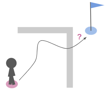
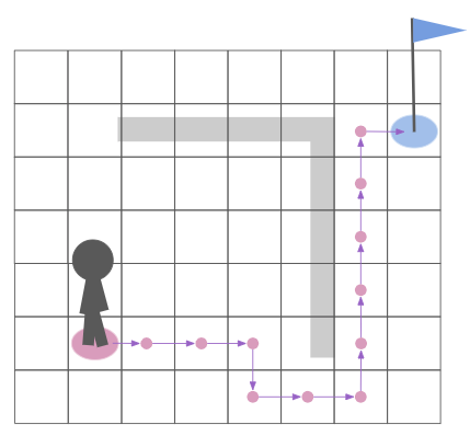
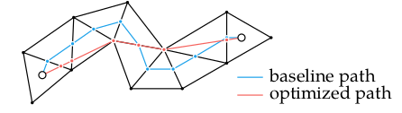
In such times of need, many of us turn to A*, in which we discretize our problem and make path planning about finding a sequence of discrete steps. But that only solves half the problem – we often end up with a chunky, often zig-zaggy solution:
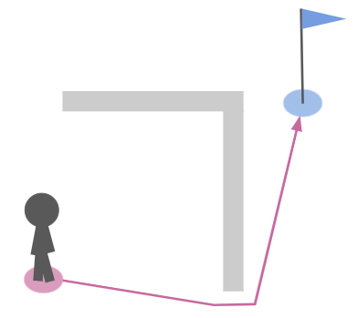
The actual shortest path doesn’t look like that. It hugs the corners and moves off-axis:
This post will cover one way to solve this problem. It will continue to leverage the power of graph algorithms like A*, but will conduct local path optimization in the second phase to get a shortest path.
Phase 1: Global, Discrete Path Planning
In the first phase, we find a coarse shortest path through a graph. Graphs are incredibly useful, and let us apply discrete approaches to the otherwise continuous world.
For this to work, the planning environment has to be represented as a graph. There are many ways to achieve this, the simplest of which is to just use a grid:
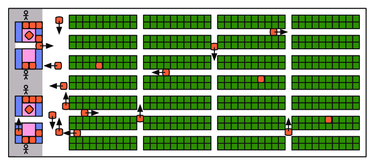
From Optimal Target Assignment and Path Finding for Teams of Agents, showing a Kiva warehouse layout.
For more general terrain it is more common to have tessellated geometry, often in the form of a navigation mesh. Below we see a path for a marine in a StarCraft 2 navmesh:

From RTS Pathfinding 3 by jdxdev, who in turn got it from Pathing it’s not a solved Problem
I first talked about navigation meshes in my post about Delaunay triangulations, and I’ve been using them to represent my game map geometry in TOOM.
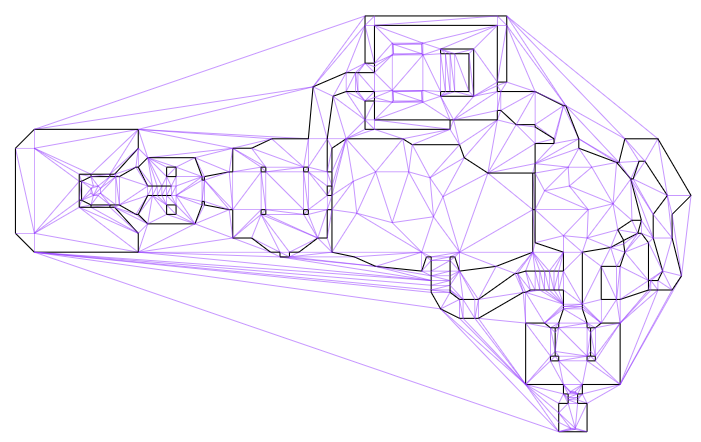
Navigation meshes, typically represented using doubly connected edge lists (DCELs), are graphs that represent both the geometry (via primal vertices and edges), and connections between faces (via dual vertices and edges). This sounds more complicated than it is. Below we see the E1M1 map from DOOM, after I’ve loaded it into a DCEL. The map walls are black and the remaining triangle edges are shown in purple:
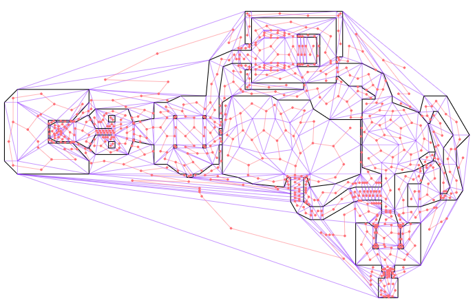
This image above only shows the primal graph, that is, the actual map geometry. The cool thing about DCELs is that they also contain a dual graph that represents connectivity between faces (triangles). Below I additionally show that dual graph in red. I’ve ignored any edges that are not traversible by the player (i.e. walls or large z changes):
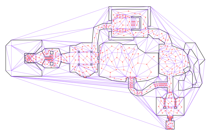
The first phase of path planning is to find the shortest path in this dual graph from our source triangle to our destination triangle. We can drop nodes that aren’t reachable:
We can run a standard graph-search algorithm on this dual graph. Each node lies at the centroid of its triangular face, and the distance between nodes can simply be the distance between the centroids. As the problem designer, you can of course adjust this as needed – maybe walking through nukage should cost more than walking over normal terrain.
In Julia this can be as simple as tossing the graph to Graphs.jl:
shortest_paths = dijkstra_shortest_paths(g, [i_src], edge_distances)
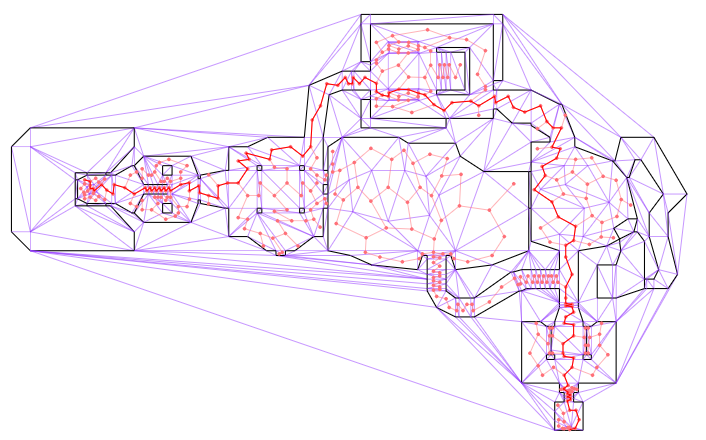
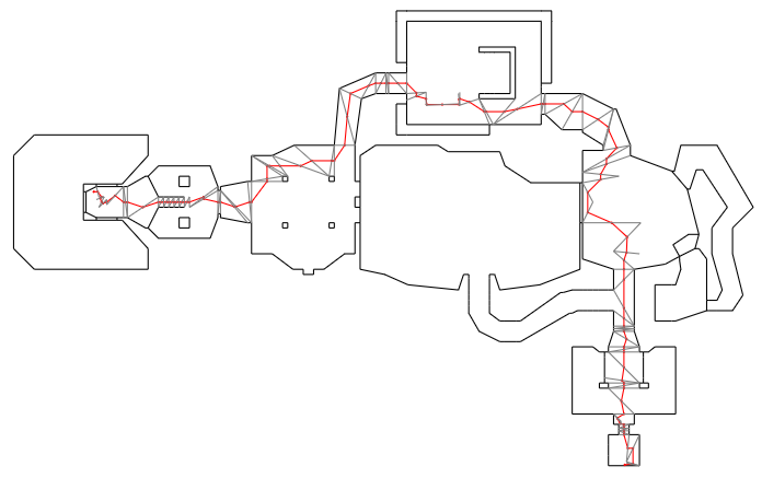
This gives us a shortest path through the triangulated environment. It is typically jagged because it can only jump between centroids. Below we see a shortest path that traverses the map:
The discrete phase of motion planning is typically very efficient, because graph search algorithms like A* or Dijkstra’s algorithm are very efficient. If our environment is more or less static, we can even precompute all shortest paths. This makes the discrete phase of motion planning very cheap.
Our problem, however, is that the resulting path is not refined. To rectify that, we need a second, local phase.
Phase 2: Local Refinement
The second phase of path planning takes our discrete path and cleans it up. Where before we were constrained to the nodes in the dual graph, in this phase we will be able to shape our path more continuously. However, we will restrain our path to continue to traverse the same sequence of faces as it did before.
Because we are restricting ourselves to the same sequence of faces, we can ignore the rest of the graph. The first thing we’ll do is switch from traversing between centroids to traversing between edges along a specific corridor. Below we show the path slightly modified (red), with traversals between the centers of the crossed faces (gray):
That is already somewhat better, but it is not good enough. Next we will shift these crossing points along the crossed edges in order to shorten the path. This can be thought if as laying down a long rubber band along the center of the traversed corridor, and then stretching it out to tighten it so that it hugs the edges. As such, this process is often called elastic band optimization or string pulling.
This is an optimization problem. How do we formulate it?
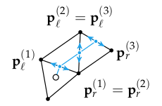
Let \(\boldsymbol{p}^{(0)}\) be our starting point, \(\boldsymbol{p}^{(n+1)}\) be our destination point, and \(\boldsymbol{p}^{(i)}\) for \(i\) in \(1:n\) be the \(n\) vertices at the edges that our path traverses. We can slide each \(\boldsymbol{p}^{(i)}\) along its edge, between its leftmost and rightmost values:
\[\boldsymbol{p}^{(i)} = \alpha_i \boldsymbol{p}_\ell^{(i)} + (1-\alpha_i)\boldsymbol{p}_r^{(i)} \]
Each interpolant \(\alpha_i\) ranges from 0 to 1. Below we depict a handful of these:
We are trying to minimize the total path length, which is the sum of the distances between sequential points:
\[\sum_{i=0}^n \| \boldsymbol{p}^{(i+1)} – \boldsymbol{p}^{(i)} \|_2\]
which in 2D is just:
\[\sum_{i=0}^n \sqrt{(\boldsymbol{p}^{(i+1)}_x – \boldsymbol{p}^{(i)}_x)^2 + (\boldsymbol{p}^{(i+1)}_y – \boldsymbol{p}^{(i)}_y)^2}\]
Our optimization problem is thus:
\[\begin{aligned}\underset{\boldsymbol{\alpha}_{1:n}}{\text{minimize}} & & \sum_{i=0}^n \| \boldsymbol{p}^{(i+1)} – \boldsymbol{p}^{(i)} \|_2 \\ \text{subject to} & & \boldsymbol{p}^{(i)} = \alpha_i \boldsymbol{p}_\ell^{(i)} + (1 – \alpha_i) \boldsymbol{p}_r^{(i)} \\ & & \boldsymbol{0} \leq \boldsymbol{\alpha} \leq \boldsymbol{1} \end{aligned}\]
This problem is convex because \(\| \boldsymbol{p}^{(i+1)} – \boldsymbol{p}^{(i)} \|_2\) is convex and the sum of convex functions is convex, the first constraint is linear (which is convex), and the inequality constraints are simple inequality constraints. We can thus solve this problem exactly.
In a game engine or robotics product we might roll our own solver, but here I’m just going to use Convex.jl:
α = Variable(n)     # interpolants
ps = Variable(2, n) # optimized points, including endpoints

problem = minimize(sum(norm(ps[:,i+1] - ps[:,i]) for i in 1:n-1))
for i in 1:n
    problem.constraints += ps[:,i] == p_ls[i] + α[i]*(p_rs[i] - p_ls[i])
end
problem.constraints += α >= 0
problem.constraints += α <= 1

solve!(problem, () -> ECOS.Optimizer(), verbose=false, silent_solver=true)

α_val = evaluate(α)
ps_opt = evaluate(ps)
Easy!
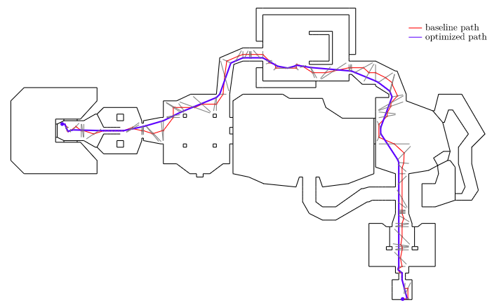
Solving our optimization problem gives us our locally-optimized shortest path:
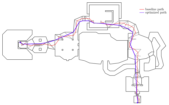
We can see how the optimized path hugs the corners and walls and heads straight across open areas. That is exactly what we want!
Agents have Width
Okay, so this gives us an optimized path, but it treats our robot / drone / enemy unit as a point mass. Our agents typically are not point masses, but have some sort of width to them. Can we handle that?
Let’s treat our agent as being a circle with radius \(r\). You can see such a circle in the earlier image for the StarCraft 2 marine.
We now modify both phases of our path planning algorithm. Phase 1 now has to ignore edges that are not at least \(2r\) across. Our agent cannot fit through anything more narrow than that. We set the path traversal cost for such edges to infinity, or remove them from the graph altogether.
Phase 2 has the more radical change. We now adjust the leftmost and rightmost points \(\boldsymbol{p}_\ell^{(1:n)}\) and \(\boldsymbol{p}_r^{(1:n)}\) to be a distance \(r\) from the line segment endpoints. This reflects the fact that our agent, with radius \(r\), cannot get closer than \(r\) to the edge of the crossed segment.
Below we show an optimized path using a small player radius. We can see how the new path continues to try to hug the walls, but maintains at least that fixed offset:
Notice that this naive augmentation introduced a few artifacts into the smoothed path, particularly near the start and end vertices. This stems from the fact that the map geometry in those location includes edges that are not actually constrained by walls on both sides. For example, the room in the bottom right has some extra triangles in order to be able to carve out that exit sign in the ceiling. It doesn’t actually hamper movement:
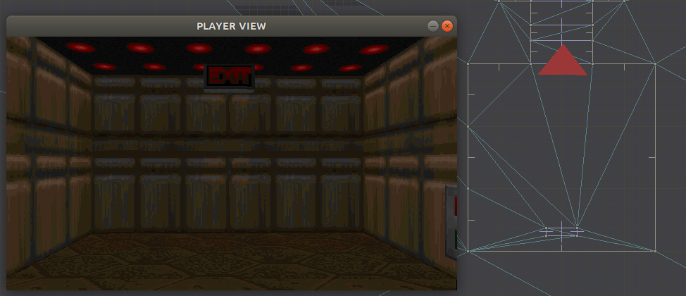
This can be fixed by using a navigation mesh that more accurately reflects player navigation. In this case, we’d remove the exit sign from the nav mesh and end up with an exit room where every edge has vertices that end at the walls.
Conclusion
This post covered a method for path planning applicable to basic robotics motion planning or for AI path planning in video games. It is a two-phase approach that separates the problem into broadly finding the homotopy of the shortest path (which side of a thing to pass on) and locally optimizing that path to find the best continuous path within the identified corridor. This method of breaking down the problem often shows up when tackling complicated problems – a discrete solver is often better at the big-picture and a local optimizer is often better for (often much-needed) local refinement.
There are many variations to the path planning problem. For example, path planning for a robot car may require restricting our path to allow for a certain turning radius, and path planning for an airplane may require planning in 3D and restricting our climb or descent rates. We may wish to minimize things other than the path distance, such as the amount of energy required, or find the shortest path that gets us there within a given energy budget. The real world is full of complexity, and having the necessary building blocks to construct your problem and the various tools at your disposal to solve them in the way that makes most sense for you makes all the difference.