One of the most interesting parts of the Convex Optimization lectures by Stephen Boyd was the realization that (continuous) optimization more-or-less boils down to repeatedly solving Ax = b. I found this quite interesting and thought I’d write a little post about it.
Constrained Optimization
An inequality-constrained optimization problem has the form:
\[\begin{aligned}\underset{\boldsymbol{x}}{\text{minimize}} & & f(\boldsymbol{x}) \\ \text{subject to} & & \boldsymbol{g}(\boldsymbol{x}) \leq \boldsymbol{0}\end{aligned}\]
One popular algorithm for solving this problem is the interior point method, which applies a penalty function that prevents iterates \(\boldsymbol{x}^{(k)}\) from becoming infeasible. One common penality function is the log barrier, which transforms our constrained optimization problem into an unconstrained optimization problem:
\[\underset{\boldsymbol{x}}{\text{minimize}} \enspace f(\boldsymbol x) \> – \> \frac{1}{\rho}
\sum_i \begin{cases}
\log\left(-g_i(\boldsymbol x)\right) & \text{if } g_i(\boldsymbol x) \geq -1 \\
0 & \text{otherwise}
\end{cases}\]
or even just
\[\underset{\boldsymbol{x}}{\text{minimize}} \enspace f(\boldsymbol x) \> – \> \frac{1}{\rho}
\sum_i \log\left(-g_i(\boldsymbol x)\right)\]
The penalty scalar \(\rho > 0\) starts small and is increased as we iterate, reducing the penalty for approaching the constraint boundary.
We thus solve our constrained optimization problem by starting with some feasible \(\boldsymbol x^{(0)}\) and then solving a series of unconstrained optimizations. So the first takeaway is that constrained optimization is often solved with iterated unconstrained optimization.
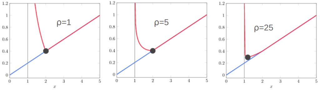
Here we see the an objective function (blue) constrained with \(x \geq 1\) (gray line). The red line shows the penalized surrogate objective. As we increase \(\rho\) and optimize, our solution moves closer and closer to \(x = 1\).
Unconstrained Optimizaton
We have found that constrained optimization can be solved by solving a series of unconstrained optimization problems.
An unconstrained optimization problem has the form:
\[\begin{aligned}\underset{\boldsymbol{x}}{\text{minimize}} & & f(\boldsymbol{x}) \end{aligned} \]
If \(f\) is continuous and twice-differentiable, we can solve this problem with Newton’s method. Here we fit a quadratic function using the local gradient and curvature and use its minimum (which we can solve for exactly) as the next iterate:
\[\boldsymbol x^{(k+1)} = \boldsymbol x^{(k)} \> – \> \boldsymbol H(\boldsymbol x^{(k)})^{-1} \nabla f(x^{(k)})\]
Continuous functions tend to become bowl-shaped close to their optimas, so Newton’s method tends to converge extremely quickly once we get close. Here is how that looks on the banana function:

What this means is that unconstrained optimization is done by repeatedly calculating Newton steps. Calculating \(\boldsymbol H(\boldsymbol x^{(k)})^{-1} \nabla f(x^{(k)})\) is the same as solving Ax = b:
\[\boldsymbol H\boldsymbol d = \nabla f\]
Well alrighty then, optimization is indeed a bunch of Ax = b.
What does this Mean
There are several takeaways.
One is that its nice that complicated things are just made up of simpler things that we can understand. One can take comfort in knowing that the world is understandable.
Another is that we should pay a lot of attention to how we compute Ax = b. Most of our time spent optimizing is spent solving Ax = b. If we can do that more efficiently, then we can optimize a whole lot faster.
Estimating Solve Times
How long does it take to solve Ax = b? Well, that depends. Let’s say we’re naive, and we have a random \(n \times n\) matrix \(\boldsymbol A\) and a random vector \(\boldsymbol b\). How fast can our computers solve that?
Well, it turns out that my laptop can solve a random \(1000 \times 1000\) linear system in about 0.35s:
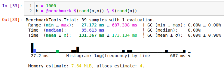
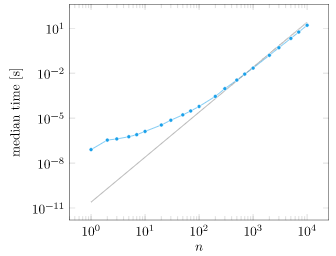
We can plot the computation time vs. matrix size:
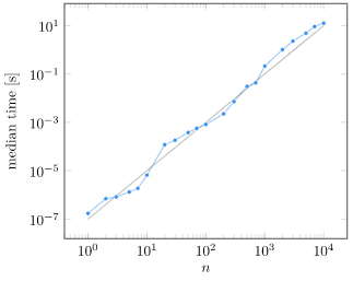
At first glance, what we see is that yes, computation grows as we increase \(n\). Things get a little fishy though. That trend line is \(n^2/10^7\), which is not the \(O(n^2)\) growth that we expected. What is going on?
While Julia itself is running single-threaded, the underlying BLAS library can use up to 8 threads:
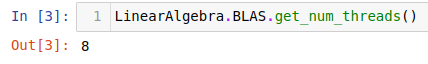
Our system is sneakily making things more efficient! If we force BLAS to be single-threaded, we get the \(O(n^3)\) growth we expected after about \(n=200\) (Thank you Julia Discourse!):
What we’ve learned is pretty important – there are speedups to be had that go beyond traditional big-O notation. If you have an optimization problem, chances are that multithreading and SIMD can speed things up for you. If you have a really large optimization problem, maybe you can distribute it across multiple machines (Proximal methods, for example, are often amenable to this).
We also learned how mind-bogglingly fast linear algebra is, even on a single thread. Think about how long it would take you to manually solve Ax = b for \(n=2\) with pen and paper, and how fast the same operation would take on your machine.
If it takes 100 Newton iterates to solve an unconstrained optimization problem, then you can solve a problem with a thousand variables in 3.5s. Multiply that by another 100 for a constrained optimization problem, and you’re looking at solving a constrained optimization problem with \(n=1000\) in under 6 minutes (and often in practice, much faster).
We live in an era where we can solve extremely large problems (GPT-4 is estimated to have 1.7 billion parameters), but we can also solve smaller problems really quickly. As engineers and designers, we should feel empowered to leverage these capabilities to improve everything.
Special Structure
Appendix C of Convex Optimization talks a lot about how to solve Ax = b. For starters, generally solving \(\boldsymbol A \boldsymbol x = \boldsymbol b\) for an arbitrary \(\boldsymbol A \in \mathbb{R}^n\) and \(\boldsymbol b \in \mathbb{R}^n\) is \(O(n^3)\). When we’re using Newton’s method, we know that the Hessian is symmetric and positive definite, so we can compute the Cholesky decomposition of \(\boldsymbol A = \boldsymbol F^\top \boldsymbol F\). Overall, this takes about half as many flops as Gaussian elimination [source].
There are a bunch of other types of structure that we can take advantage of when we know that it exists. The most obvious is when \(\boldsymbol A\) is diagonal, in which case solving Ax = b is \(O(n)\).
One particularly interesting example is when \(\boldsymbol A\) has arrow structure:
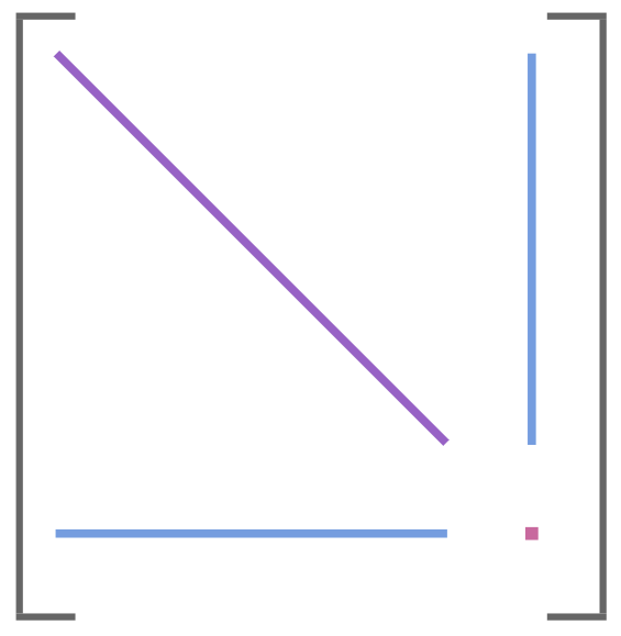
When this happens, we have to solve:
\[\begin{bmatrix} \boldsymbol A & \boldsymbol B \\ \boldsymbol B^\top & \boldsymbol C \end{bmatrix} \begin{bmatrix} \boldsymbol x \\ \boldsymbol y \end{bmatrix} = \begin{bmatrix}\boldsymbol b \\ \boldsymbol c\end{bmatrix}\]
where \( \boldsymbol A\) is diagonal, block-diagonal, or banded; \(\boldsymbol B\) is long and narrow; and \(\boldsymbol C\) is dense but comparatively small.
Solving a system with arrow structure can be done by first solving \(\boldsymbol A \boldsymbol u = \boldsymbol b\) and \(\boldsymbol A \boldsymbol V = \boldsymbol B\), which are both fast because we can exploit \( \boldsymbol A\)’s structure. Expanding the top row and solving gives us:
\[\boldsymbol x = \boldsymbol A^{-1} \left( \boldsymbol b – \boldsymbol B \boldsymbol y \right) = \boldsymbol u \> – \boldsymbol V \boldsymbol y\]
We can substitute this into the bottom row to get:
\[\begin{aligned} \boldsymbol B^\top \boldsymbol x + \boldsymbol C \boldsymbol y & = \boldsymbol c \\ \boldsymbol B^\top \left( \boldsymbol u \> – \boldsymbol V \boldsymbol y \right) + \boldsymbol C \boldsymbol y & = \boldsymbol c \\ \left( \boldsymbol C – \boldsymbol B^\top \boldsymbol V\right) \boldsymbol y & = \boldsymbol c \> – \boldsymbol B^\top \boldsymbol u\end{aligned}\]
Having solved that dense system of equations for \(\boldsymbol y\), we can back out \(\boldsymbol x\) from the first equation and we’re done.
You might think that arrow structure is a niche nicety that never actually happens. Well, if you look at how packages like Convex.jl, cvx, and cvxpy solve convex optimization problems, you’ll find that they expand and transform their input problems into a partitioned canonical form:
\[\begin{aligned}\underset{\boldsymbol x^{(1)}, \ldots, \boldsymbol x^{(k)}}{\text{minimize}} & & d + \sum_{i=1}^k \left(c^{(i)}\right)^\top \boldsymbol x^{(i)} \\ \text{subject to} & & \boldsymbol x^{(i)} \in \mathcal{S}^{(i)} \enspace \text{for } i \text{ in } \{1, \ldots, k\}\\ & & \sum_{i=1}^k \boldsymbol A^{(i)} \boldsymbol x^{(i)} = \boldsymbol b\end{aligned}\]
If we apply an interior point method to this:
\[\begin{aligned}\underset{\boldsymbol x}{\text{minimize}} & & d + \boldsymbol c^\top \boldsymbol x + \frac{1}{\rho} p_\text{barrier}(\boldsymbol x) \\ \text{subject to} & & \boldsymbol A^\top \boldsymbol x = \boldsymbol b\end{aligned}\]
we can apply a primal-dual version of Newton’s method that finds a search direction for both \(\boldsymbol x\) and the dual variables \(\boldsymbol \mu\) by solving:
\[\begin{bmatrix} \nabla^2 p_\text{barrier}(\boldsymbol x) & \boldsymbol A^\top \\ \boldsymbol A & \boldsymbol 0\end{bmatrix} \begin{bmatrix}\Delta \boldsymbol x \\ \boldsymbol \mu \end{bmatrix} = – \begin{bmatrix}\rho \boldsymbol c + \nabla p_\text{barrier}(\boldsymbol x) \\ \boldsymbol A \boldsymbol x – \boldsymbol b\end{bmatrix}\]
Wait, what is that we see here? Not only does this have arrow structure (The Hessian matrix \(\nabla^2 p_\text{barrier}(\boldsymbol x)\) is block-diagonal), but the tip of the arrow is zero! We can thus solve for the Newton step very efficiently, even for very large \(n\).
So this esoteric arrow-structure thing turns out to be applicable to general convex optimization.
Conclusion
If you take a look at university course listings, there is a clear pattern of having classes for “Linear X” and “Nonlinear X”. For example, “EE263: Introduction to Linear Dynamical Systems” and “E209B Advanced Nonlinear Control”. You learn the linear version first. Why? Because we’re really good at solving linear problems, so whenever a problem can be framed or approximated in a linear sense, we’ve either solved it that way first or found its easiest to teach it that way first. Anything can be locally approximated by a 1st-order Taylor series and we can just work with a linear system of equations.
I love that insight, but I also love the implication that it has. If we can understand how to work with linear systems, how to exploit their structure and how to solve them quickly to sufficient accuracy, then we can speed up the solution of pretty much any problem we care about. That means we can solve pretty much any problem we care about better, more often, to a higher-degree of precision, and thereby make the world a better place.