Algorithms for Optimization covers Differential Evolution in its chapter on population methods. It is fairly easy to specify what it does, but the combination of things it does is somewhat strange, and it isn’t all that obvious why it would work, or work particularly well. That being said, there is plenty of support for Differential Evolution in the literature, so I figured there probably is a method to this method’s madness. We’re in the process of updating the textbook for a 2nd edition, so in this post I’ll spend some time trying to build more intuition behind Differential Evolution to better present it in the text.
The Algorithm
Differential Evolution is a derivative-free population method. This means that instead of iteratively improving a single design, it iteratively improves a bunch of designs, and doesn’t need the gradient to do so. The individual updates make use of other individuals in the population. An effective population method will tend to converge its individuals on the (best) local minima of the objective function.
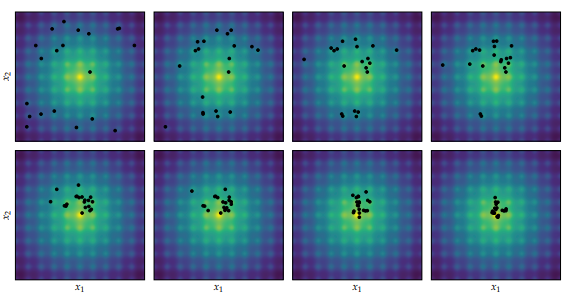
Differential Evolution applied to the Ackley function, proceeding left to right and top to bottom. Image from Algorithms for Optimization published by the MIT Press.
In each iteration, a new candidate individual \(\boldsymbol{x}’\) is created for every individual \(\boldsymbol{x}\) of the population. If the new candidate individual has a lower objective function value, it will replace the original individual in the next generation.
We first construct an interim individual \(\boldsymbol{z}\) using three randomly sampled and distinct other population members:
\[\boldsymbol{z} = \boldsymbol{a} + w \cdot (\boldsymbol{b} – \boldsymbol{c})\]
where \(w\) is a scalar weight.
The candidate design \(\boldsymbol{x}’\) is created via uniform crossover between \(\boldsymbol{z}\) and \(\boldsymbol{x}\), which just means that each component has a probability \(p\) of coming from \(\boldsymbol{z}\) and otherwise comes from \(\boldsymbol{x}\).
This is really easy to code up:
function diff_evo_step!(
    population, # vector of designs
    f,          # objective function
    p,          # crossover probability
    w)          # differential weight

    n, m = length(population[1]), length(population)
    for x in population
        a, b, c = sample(population, 3, replace=false)
        z = a + w*(b-c)
        x′ = x + (rand(m) .< p).*(z - x)
        if f(x′) < f(x)
            x[:] = x′
        end
    end
    return population
end
What I presented above is a slight simplification to the normal way Differential Evolution is typically shown. First, while my implementation samples three distinct members of the population for \(\boldsymbol{a}\), \(\boldsymbol{b}\), and \(\boldsymbol{c}\), it does not guarantee that they are distinct from \(\boldsymbol{x}\). They will pretty much always be distinct from \(\boldsymbol{x}\) for sufficiently large population sizes, and if not it isn’t all that detrimental.
Second, the standard way to define Differential Evolution always forces at least one component to mutate. This isn’t important if the crossover probability is large enough in comparison to the number of components, but in practice users have found that a very low, or even zero, crossover probability with one guaranteed mutation works best for many objective functions.
What is Going On
Differential Evolution is weird. Or at the very least, its unintuitive. Let’s break it down.
The algorithm proceeds by replacing individuals with new candidate individuals if they are better. So far so good.
The candidate individuals are formed by three things:
- a baseline individual \(\boldsymbol{a}\)
- a perturbation formed by the difference \(w\cdot(\boldsymbol{b} – \boldsymbol{c})\)
- uniform crossover
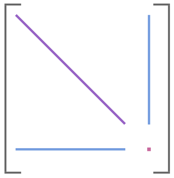
Differential Evolution gets its name from the second bullet – the difference between individuals. This is its secret sauce. Its nice in that it provides a natural way to take larger steps at the start, when the population is really spread out and hasn’t found local minima, and smaller steps later on when the population is concentrated around a few specific regions:
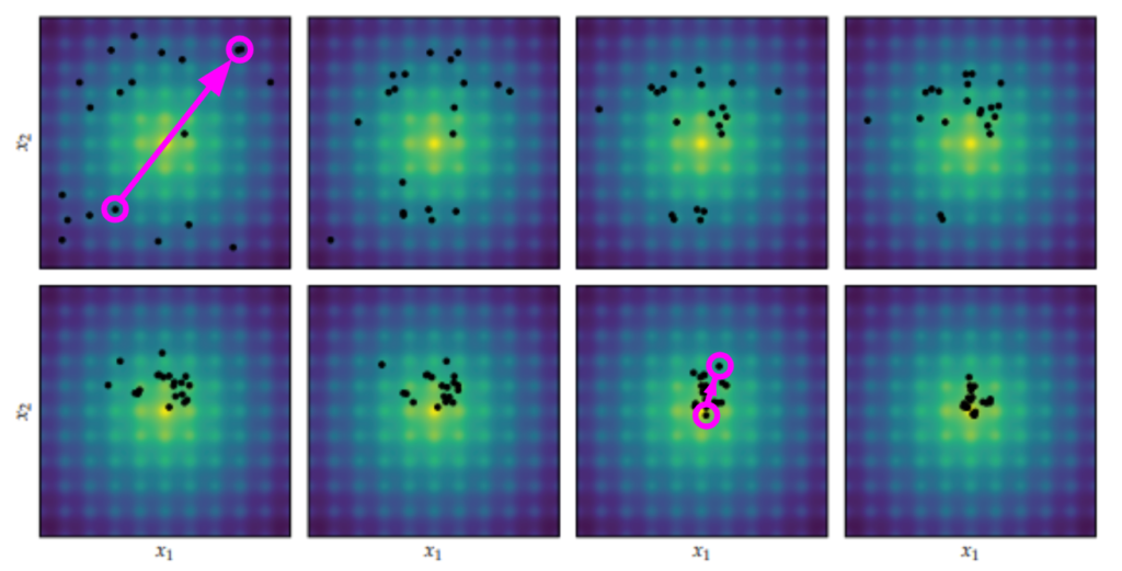
We can run a version of Differential Evolution that only has this differential, using \(\boldsymbol{x}’ = \boldsymbol{a} + w \cdot (\boldsymbol{b} – \boldsymbol{c})\). If we do that, we’ll get design improvements, but they’ll be local to the current individual. Including the baseline individual is going to do better:
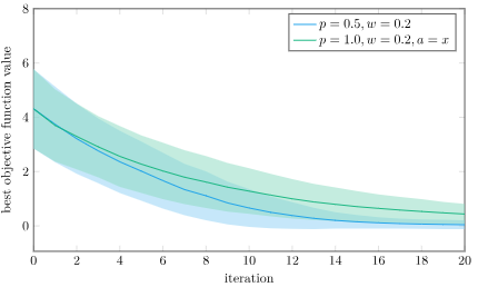
The mean best objective function value and 1 standard deviation intervals using Differential Evolution and pure differential on the Ackley function, over 1000 trials. I’m using \(w = 0.2\) to exaggerate the effect.
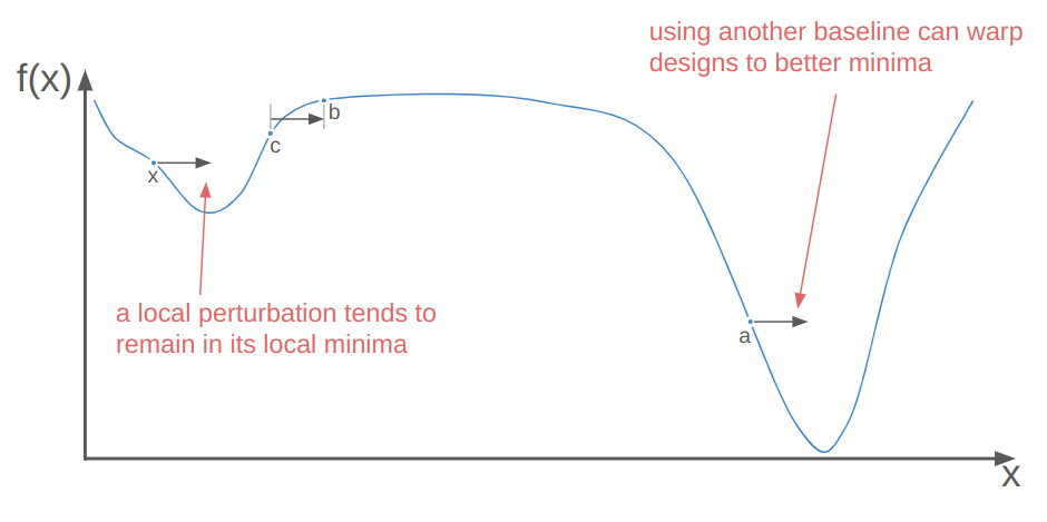
Local perturbations alone are often insufficient to get individuals out of local minima to better local minima. This is where the baseline individual \(\boldsymbol{a}\) comes in. Perturbing off of a different individual than \(\boldsymbol{x}\) means we could be substituting \(\boldsymbol{x}\) with a perturbed individual in a better local minima. When that happens, we’re basically warping \(\boldsymbol{x}\) to that better minima:
So that’s where \(\boldsymbol{a} + w \cdot (\boldsymbol{b} – \boldsymbol{c})\) comes from. What about uniform crossover? Let’s run an experiment.
Below I show the average and \(\pm 1\) standard deviation on the best objective function value vs. iteration for 1000 trials on a bunch of different algorithm variations on the Ackley function:
- no perturbation (p=0.5, w=0.0)
- no baseline individual (p=0.5, w=0.5, a=x)
- baseline Differential Evolution (p=0.5, w=0.5)
- high mutation rate (p=0.9, w=0.5)
- guaranteed crossover (p=1.0, w=0.5)
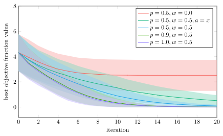
Without perturbations (w=0.0) we can’t really explore the space. We’re only looking at coordinate values that exist in our initial population. Its no surprise that that one does poorly.
Using just the baseline individual is the next-worst, because that one can’t as effectively jump individuals to new regions.
The top three performers are all Differential Evolution with varying mutation rates. We find that higher mutation rates in uniform crossover perform best. In fact, our best performance doesn’t use crossover at all, but just directly uses \(\boldsymbol{x}’ = \boldsymbol{z}\). Do we even need uniform crossover?
This table from Differential Evolution – A Simple and Efficient Heuristic for Global Optimization over Continuous Spaces shows the parameters they used on a fairly large test suite of objective functions:
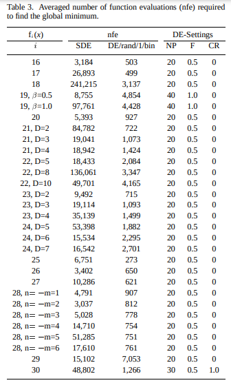
The CR column gives the crossover probability. Its basically always zero! Recall that in official implementations, crossover in Differential Evolution is guaranteed to mutate at least one component.
According to Differential Evolution: A Practical Guide to Global Optimization, this paper somewhat confused the community, because functions tended to either be solved best with \(p \approx 0\) or with \(p \approx 1\). It wasn’t until later that people made the connection that the functions that were solved with \(p \approx 0\) were decomposable, and the functions with \(p \approx 1\) were not.
A function is decomposable if it can be written as a sum of functions using distinct subsets of the inputs, such as:
\[f(\boldsymbol{x}) = \sum_i f^{(i)}(x_i)\]
When this is the case, we can improve individual components in isolation without having to be in-sync with the other components. Small mutation rates are reliable, because we can just reliably adjust a few components at a time and step our way to a minimum. By changing fewer components we have a smaller chance of messing something else up.
Most of the interesting objective functions have a high degree of coupling, and we can’t get away with optimizing some variables in isolation. For example, a neural network mixes its inputs in a convoluted manner. In order to make progress we often have to step in multiple component directions at the same time, which for Differential Evolution requires a higher crossover probability.
Optimizing Decomposable and Non-decomposable Functions
Let’s run another experiment. We’ll again do 1000 trials each (population size 20) with a bunch of versions of Differential Evolution. In the first trial, we’ll optimize a decomposable function, 10 parallel copies of Ackley’s function (making this a 20-dimensional optimization problem):
n_copies = 10
f = x -> sum(100*(x[2i-1]^2-x[2i])^2 + (1-x[2i-1])^2 for i in 1:n_copies)
We’re going to vary the mutation rate. If our results match with the literature, we expect very low mutation rates to do better.
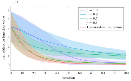
We do indeed find that low mutation rates do better. In fact, a mutation rate of zero with one guaranteed mutation is the best, closely followed by \(p = 0.1\). This does well because taking a small step in just one or two axes can more reliably lead to a win rather than moving in a bunch of axes, and this “knowledge” gained in one individual can easily be copied to other individuals to improve them too.
We can do another experiment with a non-decomposable function, in this case the xor problem. Let’s optimize some basic 2-layer feedforward neural networks. These networks have 21 parameters, so this is a 21-parameter optimization problem:
relu(x) = max(x,0.0)
sigmoid(x) = 1/(1+exp(-x))

function binary_cross_entropy(y_true, y_pred; ϵ=1e-15)
    y_pred = clamp.(y_pred, ϵ, 1-ϵ)
    return -mean(y_true .* log.(y_pred) + (1.-y_true) .* log.(1.-y_pred))
end

# xor problem
f = x -> begin
    inputs = randn(2,10)
    W1 = reshape(x[1:10], (5,2))
    b1 = x[11:15]
    W2 = reshape(x[16:20], (1,5))
    b2 = x[21]

    hidden = relu.(W1*inputs .+ b1)
    y_pred = sigmoid.(W2*hidden .+ b2)

    truth_values = inputs .> 0.0
    y_true = .!=(truth_values[1, :], truth_values[2, :])

    return binary_cross_entropy(y_true, y_pred)
end
This optimization problem is not decomposable. Taking steps in only one axis at a time is less likely to lead to significant improvements.
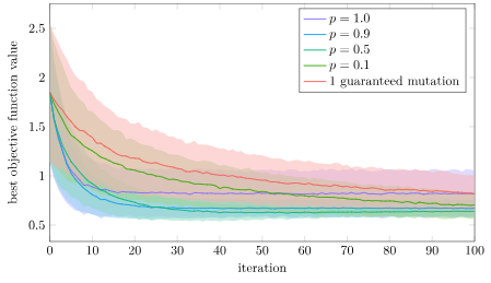
Again, that is what we see! Here the single guaranteed mutation is the worst. Interestingly, full crossover with \(p=1.0\) is initially pretty good but then tapers off, so there does appear to be some advantage to some crossover randomness. The lowest loss is most consistently achieved with \(p=0.5\), but \(p=0.9\) does nearly as well.
Why is full crossover not as good? I suspect that version will more quickly concentrate its populations into local regions, whereas having some stochasticity spreads the populations out more. Let’s plot the mean pairwise distance in the population for this experiment:
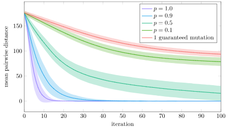
Yup! That’s exactly what we see. With full crossover, our population prematurely converges in about 20 iterations. With \(p=0.9\) it also converges pretty quick, but it apparently has enough time to find a better solution. The other crossover rates are able to avoid that premature convergence.
Conclusion
So now we know a thing or two about what makes Differential Evolution work. To recap, it uses:
- the differential between two individuals to provide perturbations, which let us explore
- this differential automatically produces smaller perturbations as the population converges
- applies the perturbation to a baseline individual which can automatically warp designs to more favorable regions
- uses uniform crossover to either
- \(p \approx 0\) force steps in a small set of coordinates; useful for separable functions
- \(p \geq 0.5\) allow for steps in many coordinates, while preventing premature convergence
So all of the ingredients have their place! Now its time to condense these learnings and add them to the next edition of the textbook.
Cheers.