This month I decided to take a break from my sidescroller project and instead properly attend to transformers (pun intended). Unless you’ve been living under a rock, you’ve noticed the rapid advanced of AI in the last year and the advent of extremely large models like ChatGPT 4 and Google Gemini. These models, and pretty much every other large and serious application of AI nowadays, are based on the transformer architecture first introduced in Attention is All You Need. So this post is about transformers, how and roughly why they work, and how to write your own.

The Architecture

The standard depiction of the transformer architecture comes from Figure 1 of Attention is All You Need:

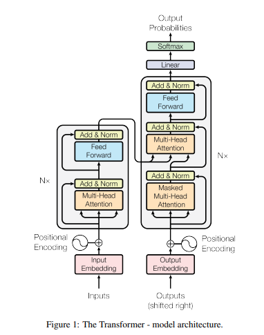
I initially found this image difficult to understand. Now that I’ve implemented my own transformer from scratch, I’m actually somewhat impressed by its concise expressiveness. That’s appropriate for a research paper where information density is key, but I think we can do better if we’re explaining the architecture to someone.

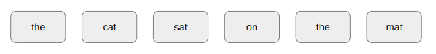
Transformers at base operate on tokens, which are just discrete items. In effect, if you have 5 tokens, then you’re talking about having tokens 1, 2, 3, 4, and 5. Transformers first became popular when used on text, where tokens represents words like “potato” or fragments like “-ly”, but they have since been applied to chunks of images, chunks of sound, simple bits, and even discrete states, actions, and rewards. I think words are the most intuitive to work with, so let’s go with that.

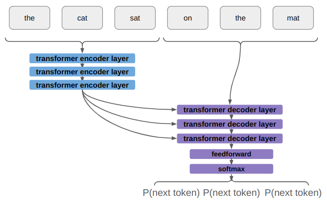
Transformers predict the next token some given all of the tokens that came before:

\[P(x_{t} \mid x_{t-1}, x_{t-2}, \ldots)\]

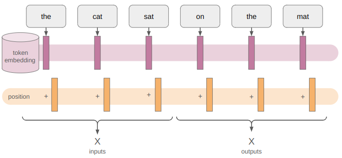
For example, if we started a sentence with “the cat sat”, we might want it to produce a higher likelihood for “on” than “potato”. Conceptually, this looks like:

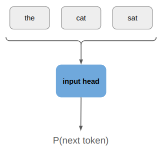
The output probability distribution is just a Categorical distribution over the \(n\) possible tokens, which we can easily produce with a softmax layer.

You’ll notice that my model goes top to bottom whereas academia for some unfathomable reason usually depicts deep neural nets bottom to top. We read top to bottom so I’m sticking with that.

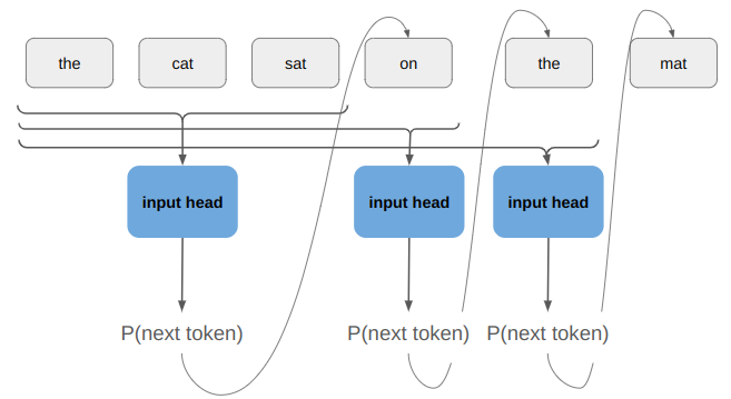
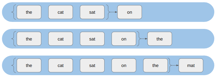
We could use a model like this to recursively generate a full sentence:

So far we’ve come up with a standard autoregressive model. Those have been around forever. What makes transformers special is that they split the inputs from the outputs such that the inputs need only be encoded once, that they use attention to help make the model resilient to how the tokens are ordered, and that they solve the problem of vanishing gradients.

Separate Inputs and Outputs

The first weird thing about the transformer architecture figure is that it has a left side and a right side. The left side receives “inputs” and the right side receives “outputs”. What is going on here?

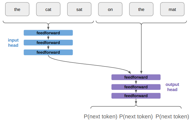
If we are trying to generate a sentence that starts with “the cat sat”, then “the cat sat” is the inputs and the subsequent tokens are the outputs. During training we’d know what the subsequent tokens are (our training set would split sentences into (input, output) pairs, such as randomly in the middle or via question/answer), and during inference we’d sample the outputs sequentially.

Conceptually, we’re now thinking about an architecture along these lines:

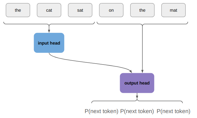
Is this weird? Yes. Why do they do it? Because it’s more efficient during training, and during inference you only need to run the input head once.

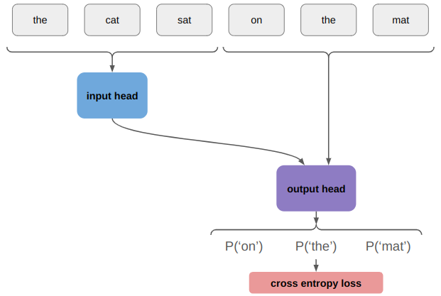
During training, we know all of the tokens and so we just stick a loss function on this to maximize the likelihood of the correct output token:

During inference, we run the encoder once and start by running the model with an empty output:

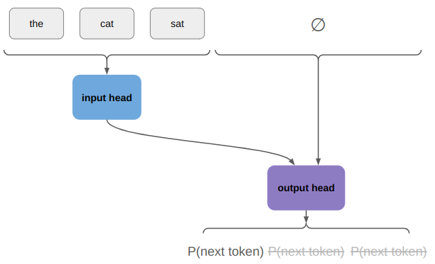
We only use the probability distribution over the first token, sample from it, and append the sampled token to our output. If we haven’t finished out sentence yet, we continue on:

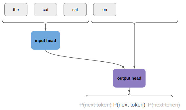
We only use the probabilistic distribution over the next token, sample from it, etc. This iterative process is auto-regressive, just like we were talking about before. (aside 1) (aside 2)

The reason I think this approach is awkward is because you’d typically want the representation of \(P(x_{t} \mid x_{t-1}, x_{t-2}, \ldots)\) to not care about whether the previous tokens were original inputs or not. That is, we want \(P(\text{the} | \text{the cat sat on})\) to be the same irrespective of whether “the cat sat on” are all inputs or whether “the cat sat” is the input and we just sampled “on”. In a transformer, they are different.

Robust to Token Ordering

The real problem that the transformer architecture solves is a form of robustness to token ordering. Let’s consider the following two input / output pairs:

the cat sat | on the mat
the yellow cat sat | on the mat

They are the same except for the extra “yellow” token in the second sentence.

If our model was made up of simple feed-forward layers, that would present a problem:

A feedforward layer contains an affine transform \(\boldsymbol{x}’ \gets \boldsymbol{A} \boldsymbol{x} + \boldsymbol{b}\) that learns a different mapping for every input. We can even write it out for three inputs:

\[\begin{matrix}x’_1 &\gets A_{11}x_1 + A_{12}x_2 + A_{13}x_3 + b_1 \\ x’_2 &\gets A_{21}x_1 + A_{22}x_2 + A_{23}x_3 + b_2 \\ x’_3 &\gets A_{31}x_1 + A_{32}x_2 + A_{33}x_3 + b_3\end{matrix}\]

If we learn something about “cat” being in the second position, we’d have to learn it all over again to handle the case where “cat” is in the third position.

Transformers are robust to this issue because of their use of attention. Put very simply, attention allows the neural network to learn when particular tokens are important in a position-independent way, such that they can be focused on when needed.

Transformers use scaled dot product attention. Here, we input three things:

a query \(\boldsymbol{q}\)
a key \(\boldsymbol{k}\)
a value \(\boldsymbol{v}\)

Each of these are vector embeddings, but they can be thought of as:

query – a representation of what we are asking for
key – how well the current token we’re looking at reflects what we’re asking for
value – how important it is that we get something that matches what we’re asking for

For example, if we have “the cat sat on the ____”, and we’re looking to fill in that last blank, it might be useful for the model to have learned a query for representing things that sit, and to value the result of that query a lot when we need to fill in a word for something that sits.

We take the dot product of the query and the key to measure how well they match: \(\boldsymbol{q}^T \boldsymbol{k}\). Each token has a key, so we end up with a measure of how well each of them matches:

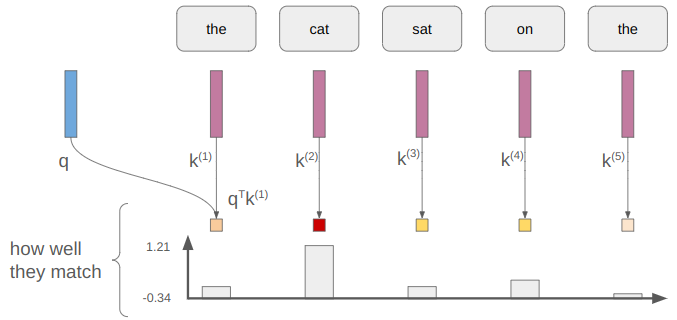
Those measures can take on any values. Taking the softmax turns these measures into values that lie in [0,1], preserving relative size: (aside)

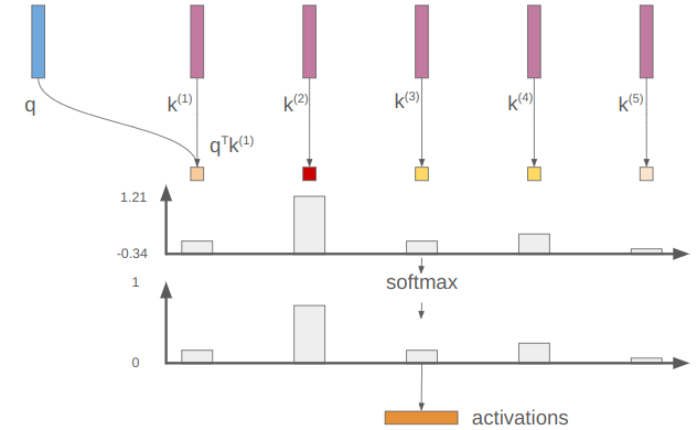
In this example, our activation vector has a large value (closer to 1) for “cat”.

Finally, we can take the dot product of our activation vector \(\boldsymbol{\alpha}\) with our value vector to get the overall attention value: \(\boldsymbol{\alpha} \cdot \boldsymbol{v}\).

Notice that where cat was in the list of tokens didn’t matter all to much. If we shift it around, but give it the same key, it will continue to produce the same activation value. Then, as long as the value is high anywhere that activation is active, we’ll get a large output.

Putting this together, our attention function for a single query \(\boldsymbol{q}\) is:

\[ \texttt{attention}(\boldsymbol{q}, \boldsymbol{k}^{(1)}, \ldots, \boldsymbol{k}^{(n)}, \boldsymbol{v}) = \texttt{softmax}\left(\boldsymbol{q}^T [\boldsymbol{k}^{(1)}, \ldots, \boldsymbol{k}^{(n)}]\right) \cdot \boldsymbol{v} \]

We can combine the keys together into a single matrix \(\boldsymbol{K}\), which simplifies things to:

\[ \texttt{attention}(\boldsymbol{q}, \boldsymbol{K}, \boldsymbol{v}) = \texttt{softmax}\left(\boldsymbol{q}^T \boldsymbol{K}\right) \cdot \boldsymbol{v} \]

We’re going to want a bunch of queries, not just one. That’s equivalent to expanding our query and value vectors into matrices:

\[ \texttt{attention}(\boldsymbol{Q}, \boldsymbol{K}, \boldsymbol{V}) = \texttt{softmax}\left(\boldsymbol{Q}^T \boldsymbol{K}\right) \boldsymbol{V} \]

We’ve basically recovered the attention function given in the paper. I just has an additional scalar term that helps keep the logits passed into softmax smaller in magnitude:

\[\texttt{attention}(\boldsymbol{Q}, \boldsymbol{K}, \boldsymbol{V}) = \texttt{softmax}\left(\frac{\boldsymbol{Q}\boldsymbol{K}^T}{\sqrt{d_k}}\right) \boldsymbol{V}\]

where \(d_k\) is the dimension of the keys — i.e. how many features long the embeddings are.

The output is a matrix that has larger entries where our queries matched tokens and our value was large. That is, the transformer learned to ask for something and extract it out if it exists.

Robust to Vanishing Gradients

The other important problem that transformers solve is the vanishing gradient problem. The previous alternative to the transformer, the recurrent neural network (RNN), tends to suffer from this issue.

A recurrent neural network represents a sequence by taking as input the current token and a latent state:

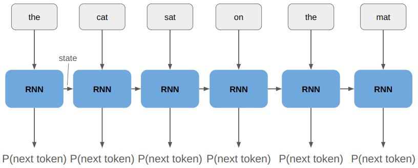
This state is referred to as the RNN’s memory.

The vanishing gradients problem arises when we try to propagate gradient information far back in time (where far can just be a few tokens). If we want the network to learn to associate “mat” with “cat”, then we need to propagate through 4 instances of the RNN:

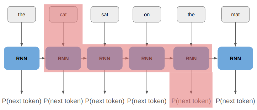
Simply put, in this example we’re taking the gradient of RNN(RNN(RNN(RNN(“cat”, state)). The chain rule tells us that the derivative of \(f(f(f(f(x))))\) is:

\[f'(x) \> f'(f(x)) \> f'(f(f(x))) \> f'(f(f(f(x))))\]

If \(f'(x)\) is smaller than 1, then we very quickly drive that gradient signal toward zero as we try to propagate it back further. The gradient vanishes!

Transformers solve this problem by having all of the inputs be mixed in the attention layers. This allows the gradient to readily flow across.

It also mitigates the problem using residual connections. These are the “skip connections” that you’ll see below. They provide a way for the gradient to flow up the network unimpeded, so it doesn’t decrease if it has to travel through a bunch of transformer layers.

Building a Transformer

Let’s use what we’ve learned and build a transformer, setting aside the fact that we haven’t covered multiheaded attention just yet. We’re going to construct the following input head:

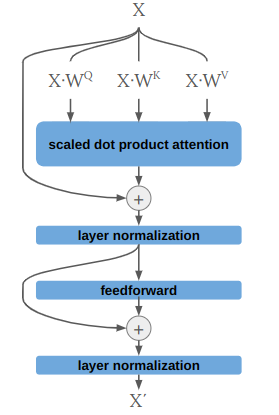
This is analogous to a single “input encoder layer” in the transformer architecture. Note that the real deal uses multiheaded attention and has dropout after each layer norm.

The trainable parameters in our input head are the three projection matrices \(\boldsymbol{W}^Q\), \(\boldsymbol{W}^K\), and \(\boldsymbol{W}^V\), as well as the learnable params in the feedforward layer. Layer normalization is simply normalization along each input vector rather than along the batch dimension, which keeps things nicely scaled.

I’m going to implement this input head in Julia, using Flux.jl. The code is remarkably straightforward and self-explanatory:

struct InputHead
    q_proj::Dense
    k_proj::Dense
    v_proj::Dense
    norm_1::LayerNorm
    affine1::Dense
    affine2::Dense
    norm_2::LayerNorm
end

Flux.@functor InputHead

function (m::InputHead)(
    X::Array{Float32, 3}) # [dim × ntokens × batch_size]

    dim = size(X, 1)

    # scaled dot product attention
    Q = m.q_proj(X) # [dim × ntokens × batch_size]
    K = m.k_proj(X) # [dim × ntokens × batch_size]
    V = m.v_proj(X) # [dim × ntokens × batch_size]
    α = softmax(Q*K'./√Float32(dim), dims=1)
    X′ = α*V

    # add norm
    X = m.norm_1(X + X′)

    # feedforward
    X′ = m.affine2(relu(m.affine1(X)))
    
    # add norm
    X = m.norm_1(X + X′)

    return X
end

Once we have this, building the rest of the simplified transformer is pretty easy. Let’s similarly define an output head:

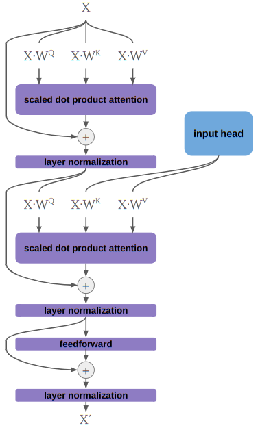
The output head is basically the same, except it has an additional attention + layer normalization section that receives its query from within the head but its keys and values from the input head. This is sometimes called cross attention, and allows the outputs to receive information from the inputs. Implementing this in Julia would be pretty straightforward, so I’m not covering it here.

In order to fully flesh out a basic transformer, we just have to define what happens at the outputs and inputs. The output is pretty simple. Its just a feedforward layer followed by a softmax:

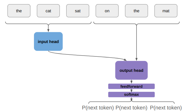
The feedforward layer both provides a chance for everything to get properly mixed (since its fully connected), but more importantly, changes the tensor dimension from the embedding size to the number tokens. The softmax then ensures that the output represents probabilities.

The inputs, by which I mean all of the tokens, have to be turned into embedding matrices. Remember that there’s only a finite set of tokens. We associate a vector embedding with each token, which we re-use every time the token shows up. This embedding can be learned, in which case its the same as having our token be a one-hot vector \(x_\text{one-hot}\) and learning some matrix \(m\times n\) matrix \(E\) where \(m\) is the embedding dimension and \(n\) is the number of tokens:

\[z = E x_\text{one-hot}\]

We then add a positional encoding to each embedding. Wait, I thought we wanted the network to be robust to position? Well yeah, it is. But knowing where something shows up, and whether it shows up before or after something else is also important. So to give the model a way to determine that, we introduce a sort of signature or pattern to each embedding. The original paper uses a sinusoidal pattern:

\[z_\text{pos encode}(i)_j = \begin{cases} \sin\left(i / 10000^{2j / j_\text{max}}\right) & \text{if } j \text{ is even} \\ \cos\left(i / 10000^{2j / j_\text{max}}\right) & \text{otherwise} \end{cases}\]

for the \(j\)th entry of the position encoding at position \(i\).

What I’m not showing here is that the original paper again uses dropout after the position encoding is added in.

Flux already supports token embeddings, so let’s just use that. We can just generate our position encodings in advance:

function generate_position_encoding(dim::Int, max_sequence_length::Int)
    pos_enc = zeros(Float32, dim, max_sequence_length)

    for j in 0:2:(dim-1)
        denominator::Float32 = 10000.0^(2.0*(j ÷ 2)/dim)
        for i in 1:max_sequence_length
            pos_enc[j+1, i] = sin(i / denominator)
        end
    end

    for j in 1:2:(dim-1)
        denominator::Float32 = 10000.0^(2.0*(j ÷ 2)/dim)
        for i in 1:max_sequence_length
            pos_enc[j+1, i] = cos(i / denominator)
        end
    end

    return pos_enc
end

The overall input encoder is then simply:

struct InputEncoder
    embedding::Embedding # [vocab_size => dim]
    position_encoding::Matrix{Float32} # [dim × n_tokens]
    dropout::Dropout
end

Flux.@functor InputEncoder

function (m::InputEncoder)(tokens::Matrix{Int}) # [n_tokens, batch_size]
    X = m.embedding(tokens) # [dim × n_tokens × batch_size]
    X = X .+ m.position_encoding
    return m.dropout(X)
end

When it gets down to it, coding this stuff up really is just like stacking a bunch of lego bricks.

We can put it all together to get a super-simple transformer:

struct Transformer
    input_encoder::InputEncoder
    trans_enc::TransformerEncoderLayer
    trans_dec::TransformerDecoderLayer
    linear::Dense # [vocab_size × dim]
end

Flux.@functor Transformer

function Transformer(vocab_size::Int, dim::Int, n_tokens::Int;
                   hidden_dim_scale::Int = 4,
                   init = Flux.glorot_uniform,
                   dropout_prob = 0.0)
    input_encoder = InputEncoder(
        Flux.Embedding(vocab_size => dim),
        generate_position_encoding(dim, n_tokens),
        Dropout(dropout_prob))
    trans_enc = TransformerEncoderLayer(dim,
        hidden_dim_scale=hidden_dim_scale,
        bias=true, init=init, dropout_prob=dropout_prob)
    trans_dec = TransformerDecoderLayer(dim,
        hidden_dim_scale=hidden_dim_scale,
        bias=true, init=init, dropout_prob=dropout_prob)
    linear = Dense(dim => vocab_size, bias=true, init=init)
    return Transformer(input_encoder, trans_enc, trans_dec, linear)
end

function (m::Transformer)(
    input_tokens::Matrix{Int},
    output_tokens::Matrix{Int}) # [n_tokens, batch_size]

    X_in = m.input_encoder(input_tokens) # [dim × n_tokens × batch_size]
    X_out = m.input_encoder(output_tokens) # [dim × n_tokens × batch_size]
    E = m.trans_enc(X_in)
    X = m.trans_dec(X_out, E)
    logits = m.linear(X) # [vocab_size × n_tokens × batch_size]
    return logits
end

Note that this code doesn’t run a softmax because we can directly use the crossentropy loss on the logits, which is often more accurate.

Running this model requires generating datasets of tokens, where each token is an integer. We pass in our batch of token inputs and our batch of token outputs, and see what logits we get.

Masking

We’ve got a basic transformer that will take input tokens and produce output logits. We can train it to the maximize the likelihood of the expected future tokens. We’ll probably be able to perform pretty well on the training set, but if we go and try to actually generate sentences, it won’t do all that well.

Why? Because the current setup allows the neural network to attend to future information.

Recall that we’re trying to predict the next token given the tokens that came before:

\[P(x_{t} \mid x_{t-1}, x_{t-2}, \ldots)\]

The way our output head is currently constructed, we’re allowing tokens there to attend all of the tokens, which includes future output tokens.

Let’s revisit our attention function for a single query \(\boldsymbol{q}\):

We want to modify the attention function such that we do not consider the keys for tokens beyond a certain index, say index \(t\). That means we want softmax to disregard those tokens. To achieve that, we need their values to be \(-\infty\):

\[ \underset{\leq t}{\texttt{attention}}(\boldsymbol{q}, \boldsymbol{k}^{(1)}, \ldots, \boldsymbol{k}^{(n)}, \boldsymbol{v}) = \texttt{softmax}\left([\boldsymbol{q}^T \boldsymbol{k}^{(1)}, \ldots, \boldsymbol{q}^T \boldsymbol{k}^{(t)}, -\infty, \ldots, -\infty]\right) \cdot \boldsymbol{v} \]

One easy way to do this is to pass in an additional mask vector that is zero for \(i \leq t\) and negative infinity otherwise:

\[ \begin{aligned}\underset{\leq t}{\texttt{attention}}(\boldsymbol{q}, \boldsymbol{k}^{(1)}, \ldots, \boldsymbol{k}^{(n)}, \boldsymbol{v}) = \texttt{softmax}( & [\boldsymbol{q}^T \boldsymbol{k}^{(1)}, \ldots, \boldsymbol{q}^T \boldsymbol{k}^{(t)}, \boldsymbol{q}^T \boldsymbol{k}^{(t+1)}, \ldots, \boldsymbol{q}^T \boldsymbol{k}^{(n)}] + \\ & [0, \ldots, 0, -\infty, \ldots, -\infty]) \cdot \boldsymbol{v}\end{aligned} \]

\[ \texttt{attention}(\boldsymbol{q}, \boldsymbol{K}, \boldsymbol{v}, \boldsymbol{m}) = \texttt{softmax}( \boldsymbol{q}^T \boldsymbol{K} + \boldsymbol{m}) \cdot \boldsymbol{v} \]

We don’t use just one query, we use a bunch. If you’re paying attention, you noticed that we actually get one query per output-head token because our query matrix is:

\[\boldsymbol{Q} = \boldsymbol{X}\cdot \boldsymbol{W}^Q\]

So we want \(\boldsymbol{q}^{(1)}\) to use \(t = 1\), \(\boldsymbol{q}^{(2)}\) to use \(t = 2\), etc. This means that when we move to attention with multiple queries, we get:

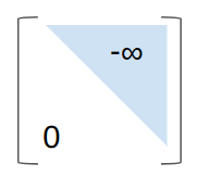
\[ \texttt{attention}(\boldsymbol{Q}, \boldsymbol{K}, \boldsymbol{V}, \boldsymbol{M}) = \texttt{softmax}\left( \frac{\boldsymbol{Q} \boldsymbol{K}^T}{\sqrt{d_k}} + \boldsymbol{M}\right) \boldsymbol{V} \]

where \(\boldsymbol{M}\) is a lookahead mask with the upper right triangle set to negative infinity:

Check out this blog post for some additional nice coverage of self-attention masks.

Are We Done Yet?

Alright, we’ve got our baby transformer and we’ve added lookahead attention. Are we done?

Well, sort of. This is the minimum amount of stuff necessary to appropriately learn something that can call itself a transformer and that will probably sort-of work. All of the concepts are there. A real transformer will be the same, just bigger.

First, it will use multi-headed rather than single-headed attention. This just means that it does single-headed attention multiple times in parallel:

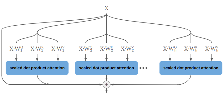
We could do that by running a \(\texttt{for}\) loop over multiple attention heads, but in practice it can be implemented by splitting our tensor into a new dimension according to the number of heads:

function (mha::MultiHeadAttention)(
    Q_in::Array{Float32, 3}, # [dim × ntokens × batch_size]
    K_in::Array{Float32, 3}, # [dim × ntokens × batch_size]
    V_in::Array{Float32, 3}, # [dim × ntokens × batch_size]
    mask::Array{Float32, 2}) # [ntokens × ntokens]

    dims = size(Q_in)
    dim = dims[1]

    # All matrices end up being [dim × ntokens × batch_size]
    Q = mha.q_proj(Q_in) # [dim × ntokens × batch_size]
    K = mha.k_proj(K_in) # [dim × ntokens × batch_size]
    V = mha.v_proj(V_in) # [dim × ntokens × batch_size]

    # Reshape to # [dim÷nheads × nheads × ntokens × batch_size]
    Q = reshape(Q, dim ÷ mha.nheads, mha.nheads, dims[2:end]...)
    K = reshape(K, dim ÷ mha.nheads, mha.nheads, dims[2:end]...)
    V = reshape(V, dim ÷ mha.nheads, mha.nheads, dims[2:end]...)

    # We're going to use batched_mul, which operates on the first 2 dimensions.
    # We want Q, K, and V to act as `nheads` separate attention heads, so we 
    # need to move the 'nheads' dimension out of the first 2 dimensions.
    Kp = permutedims(K, (3, 1, 2, 4)) # This effectively takes care of the transpose too
    Qp = permutedims(Q, (1, 3, 2, 4)) ./ √Float32(dim)
    logits = batched_mul(Kp, Qp) # [ntokens × ntokens × nheads × batch_size]

    # Apply the mask
    logits = logits .+ mask # [ntokens × ntokens × nheads × batch_size]

    # Compute the activations
    α = softmax(logits, dims=1) # [ntokens × ntokens × nheads × batch_size]

    # Run dropout on the activations
    α = mha.dropout(α) # [ntokens × ntokens × nheads × batch_size]

    # Multiply by V, again with a batched_mul
    Vp = permutedims(V, (1, 3, 2, 4))
    X = batched_mul(Vp, α)
    X = permutedims(X, (1, 3, 2, 4)) # [dim÷nheads × nheads × ntokens × batch_size]
    X = reshape(X, :, size(X)[3:end]...) # [dim × ntokens × batch_size]

    # Compute the outward projection
    return mha.out_proj(X) # [dim × ntokens × batch_size]
end

Note that in this code, the inputs are all X in the first multi-headed attention layer of the output head, whereas in the second one (called the cross attention layer), the queries Q_in are set to X whereas the keys and values are set to the output of the input head.

The other thing that a real transformer has is multiple transformer layers. That is, we repeat what we currently have as our input head and output head multiple times:

The Attention is All You Need paper used 8 parallel attention layers (attention heads) and 6 identical layers each in the encoder (input head) and decoder (output head).

Conclusion

I hope this post helps demystify the transformer architecture. They are the workhorse of modern large-scale deep learning, and its worth familiarizing yourself with them if you’re going to be working in that area. While complicated at first glance, they actually arise from fairly straightforward principles and solve some fairly practical and understandable problems. The information here should be enough to get started using them, or even roll your own from scratch.

Happy coding!

Tim Wheeler

Transformers – How and Why They Work