I recently read a fantastic blog post about Delaunay triangulations and quad-edge data structures, and was inspired to implement the algorithm myself. The post did a very good job of breaking the problem and the algorithm down, and had some really nice interactive elements that made everything make sense. I had tried to grok the quad-edge data structure before, but this was the first time where it really made intuitive sense.
This post covers more or less the same content, in my own words and with my own visualizations. I highly recommend reading the original post.
What is a Delaunay Triangulation
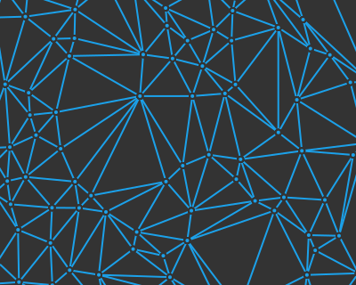
A triangulation is any breakdown of a set of vertices into a set of non-overlapping triangles. Some triangulations are better than others, and the Delaunay triangulation is a triangulation that makes each triangle as equilateral as possible. As a result, it is the triangulation that keeps all of the points in a given triangle as close to each other as possible, which ends up making it quite useful for a lot of spacial operations, such as finite element meshes.
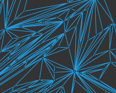
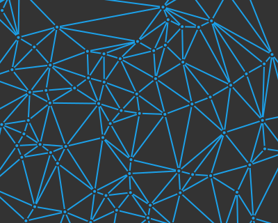
As we can see above, there are a lot of bad triangulations with a lot of skinny triangles. Delaunay triangulations avoid that as much as possible.
One of the neatest applications of these triangulations is in motion planning. In constrained Delaunay triangulation, you for all walls in your map to be edges in your triangulation, and otherwise construct a normal Delaunay triangulation. Then, your robot can pass through any edge of sufficient length (i.e., if its a wide enough gap), and you can quickly find shortest paths through complicated geometry while avoiding regions you shouldn’t enter:
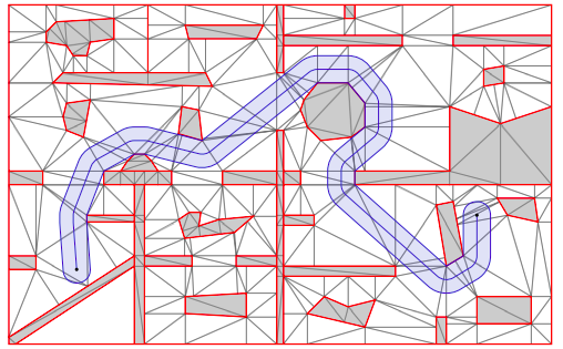
Roadmap Graphs with Arbitrary Clearance” by S. Lens and B. Boigelot
How to Construct a Delaunay Triangulation
So we want a triangulation that is as equilateral as possible. How, technically, is this achieved?
More precisely, a triangulation is Delaunay if no vertex is inside the circumcircle of any of the triangles. (A circumcircle of a triangle is the circle that passes through its three vertices).
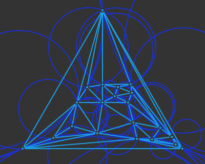
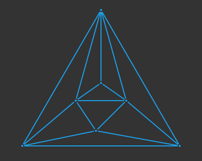
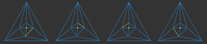
One way to construct a Delaunay triangulation for a set of points is construct one iteratively. The Guibas & Stolfi incremental triangulation algorithm starts with a valid triangulation and repeatedly adds a new point, joining it into the triangulation and then changing edges to ensure that the mesh continues to be a Delaunay triangulation:
Here is the same sequence, with some details skipped and more points added:
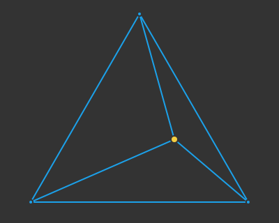
This algorithm starts with a bounding triangle that is large enough to contain all future points. The triangle is standalone, and so by definition is Delaunay:
Every iteration of the Guibas & Stolfi algorithm inserts a new point into our mesh. We identify the triangle that new point is inside, and connect edges to the new point:
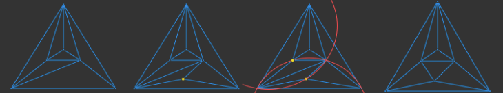
Note that in the special case where our new vertex is on an existing edge (or sufficiently close to an existing edge) we remove that edge and introduce four edges instead:
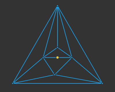
By introducing these new edges we have created three (or four) new triangles. These new triangles may no longer fulfill the Delaunay requirement of having vertices that are within some other triangle’s circumcircle.
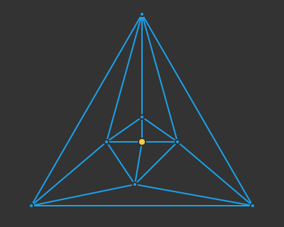
Guibas & Stolfi noticed that the only possible violations occur between the new point and those opposite its surrounding face. That is, we need only walk around the edges of the triangle (or quadrilateral) that we inserted it into, and check whether we should flip those border edges in order to preserve the Delaunay condition.
For example, for the new vertex above, we only need to check the four surrounding edges:
Here is an example where we need to flip an edge:
Interestingly, flipping an edge simply adds a new spoke to our new vertex. As such, we continue to only need to check the perimeter edges around the hub. This guarantees that we won’t propagate out and have to spend a lot of time checking edges, but instead just iterate around our one new point.
That’s one iteration of the algorithm. After that you just start the next iteration. Once you’re done adding points you remove the bounding triangle and you have your Delaunay triangulation.
The Data Structure
So the concept is pretty simple, but we all know that the devil is in the details. What really excited me about the Delaunay triangulation was the data structure used to construct it.
If we look at the algorithm, we can see what we might need our data structure to support:
- Find the triangle enclosing a new point
- Add new edges
- Find vertices across from edges
- Walk around the perimeter of a face
Okay, so we’ve got two concepts here – the ability to think about edges in our mesh, but also the ability to reason about faces in our mesh. A face, in this case, is usually a triangle, but it could also sometimes be a quadrilateral, or something larger.
The naive approach would be to represent our triangulation (i.e. mesh) as a a graph. That is, a list of vertices and a way to represent edge adjacency. Unfortunately, this causes problems. The edges would need to be ordered somehow to allow us to navigate the mesh.
The data structure of choice is called a quad-edge tree. It gives us the ability to quickly navigate both clockwise or counter-clockwise around vertices, or clockwise or counter-clockwise around faces. At the same time, quad-edge trees make it easy for new geometry to be stitched in or existing geometry to be removed.
Many of the drawings and explanations surrounding quad-edge trees are a bit complicated and hard to follow. I’ll do my best to make this explanation as tractable as possible.
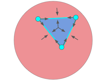
A quad-edge tree for 2D data represents a vertex mesh on a sphere:
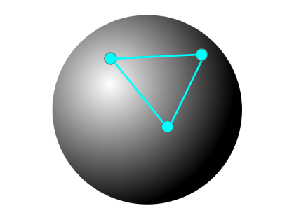
Said sphere is mostly irrelevant for what we are doing. In fact, we can think of it as very large. However, there is one important consequence of being on a sphere. Now, every edge between two vertices is between two faces. For example, the simple 2D mesh above has two faces:
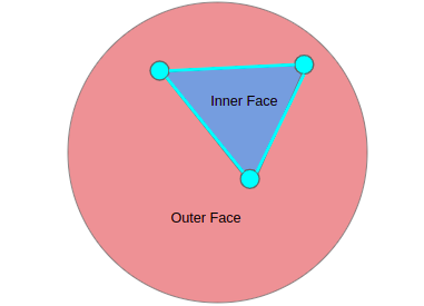
The quad-edge data structure can leverage this by associating each edge both with its two vertices and with its two faces, hence the name. Each real edge is represented as four directional edges in the quad-edge data structure: two directional edges between vertices and two directional edges between faces.
We can thus think of each face as being its own kind of special vertex:
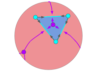
As such, the quad-edge data structure actually contains two graphs – the directed graph of mesh edges and the dual graph that connects mesh faces. Plus, both of these graphs have inter-connectivity information in that .
Okay, so pretty abstract. But, this gives us what we want. We can easily traverse the mesh by either flipping between the directed edges for a given mesh edge, or rotating around the base vertices for a given directed edge:

So now we are thinking about a special directed graph where each directed edge knows its left and right-hand neighbors and the other three directed edges that make up the edge in the original mesh:
struct QuarterEdge
    data::VertexIndex # null if a dual quarter-edge
    next_in_same_edge_on_right::QuarterEdgeIndex
    next_in_same_edge_on_left::QuarterEdgeIndex
    next_with_same_base_on_right::QuarterEdgeIndex
    next_with_same_base_on_left::QuarterEdgeIndex
end
struct Mesh
    vertices::Vector{Point}
    edges::Vector{QuarterEdge}
end
We have to update these rotational neighbors whenever we insert new edges into the mesh. It turns out we can save a lot of headache by dropping our left-handed neighbors:
struct QuarterEdge
    data::VertexIndex # null if a dual quarter-edge
    rot::QuarterEdgeIndex # next in same edge on right
    next::QuarterEdgeIndex # next with same base on right
end
We can get the quarter-edge one rotation to our left within the same edge simply by rotating right three times. Similarly, we can get the quater-edge one rotation to our left with the same base vertex by following rot – next – rot:
Now we have our mesh data structure. When we add or remove edges, we have to be careful (1) to always construct new edges using four quarter edges whose rot entries point to one another, and (2) to update the necessary next entries both in the new edge and in the surrounding mesh. There are some mental hurdles here, but it isn’t too bad.
Finding the Enclosing Triangle
The first step of every Delaunay triangulation iteration involves finding the triangle enclosing the new vertex. We can identify a triangle using a quarter edge q whose base is associated with that face. If we do that, its three vertices, in counter-clockwise order, are:
- A = q.rot.data
- B = q.next.rot.data
- C = q.next.next.rot.data
(Note that in code this looks a little different, because in Julia we would be indexing into the mesh arrays rather than following pointers like you would in C, but you get the idea).
Suppose we start with some random face and extract its vertices A, B, and C. We can tell if our new point P is inside ABC by checking whether P is to the left of the ray AB, to the left of the ray BC, and to the left of the ray CA:
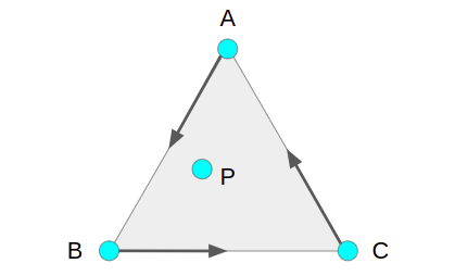
Checking whether P is left of a ray AB is the same as asking whether the triangle ABP has a counter-clockwise ordering. Conveniently, the winding of ABP is given by the determinant of a matrix:
\[\text{det}\left(\begin{bmatrix} A_x & A_y & 1 \\ B_x & B_y & 1 \\ P_x & P_y & 1 \end{bmatrix} \right)\]
If this value is positive, then we have right-handed (counter-clockwise) winding. If it is negative, then we have left-handed (clockwise) winding. If it is zero, then our points are colinear.
If our current face has positive windings then it encloses our point. If any winding is negative, the we know we can cross over that edge to get closer to our point.
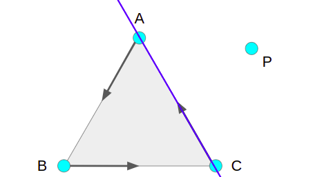
We simply iterate in this manner until we find our enclosing face. (I find this delightfully clean.)
Is a Point inside a Circumcircle
Checking whether vertices are inside circumcircles of triangles is central to the Delaunay triangulation process. The inspiring blog post has great coverage of why the following technique works, but if we want to check whether a point P is inside the circumcircle that passes through the (counter-clockwise-oriented) points of triangle ABC, then we need only compute:
\[\text{det}\left(\begin{bmatrix} A_x & A_y & A_x^2 + A_y^2 & 1 \\ B_x & B_y & B_x^2 + B_y^2 & 1 \\ C_x & C_y & C_x^2 + C_y^2 & 1 \\ P_x & P_y & P_x^2 + P_y^2 & 1 \end{bmatrix}\right)\]
If this value is positive, then P is inside the circumcircle. If it is negative, then P is external. If it is zero, then P is on its perimeter.
Some Last Implementation Details
I think that more or less captures the basic concepts of the Delaunay triangulation. There are a few more minor details to pay attention to.
First off, it is possible that our new point is exactly on an existing edge, rather than enclosed inside a triangle. When this happens, or when the new point is sufficiently close to an edge, it is often best to remove that edge and add four new edges. I illustrate this earlier in the post. That being said, make sure to never remove / split an original bounding edge. It is, after all, a bounding triangle.
Second, after we introduce the new edges we have to consider flipping edges around the perimeter of the enclosing face. To do this, we simply rotate around until we arrive back where we started. The special cases here are bounding edges, which we never flip, and edges that connect to our bounding vertices, which we don’t flip if it would produce new triangles with clockwise windings:
Once you’re done adding vertices, you remove the bounding triangle and any edges connected to it.
And all that is left as far as implementation details are concerned is the implementation itself! I put this together based on that other blog post as a quick side project, so it isn’t particularly polished. (Your mileage may vary). That being said, its well-visualized and I generally find reference implementations to be nice to have.
Conclusion
I thought the quad-edge data structure was really interesting, and I bet with some clever coding they could be really efficient as well. I really liked how solving this problem required geometry and visualization on top of typical math and logic skills.
Delaunay triangulations have a lot of neat applications. A future step might be to figure out constrained Delaunay triangulations for path-finding, or to leverage the dual graph to generate Voronoi diagrams.