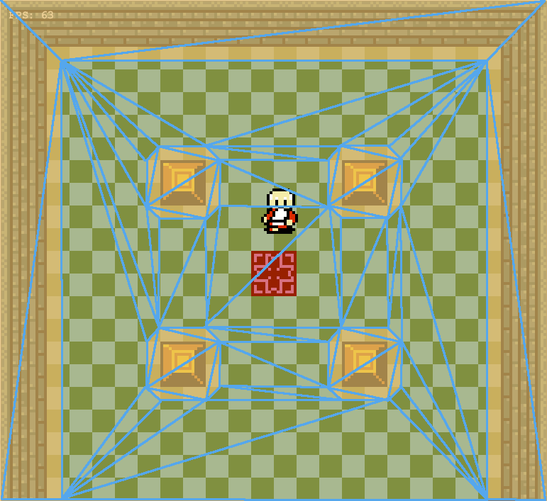
Cart Pole with Actuator Limits

In the previous post, we used an LQR controller to solve the classic cart-pole problem. There, the action space is continuous, and our controller is allowed to output any force. This leads to some very smooth control.

LQR Control

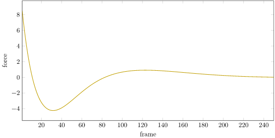
We can plot the force over time:

We can see that our force starts off at 8 N and oscillates down to about -4 N before settling down as the cart-pole system stabilizes. This raises a question – don’t real world actuators saturate? What happens if we model that saturation?

LQR with Saturation

The original LQR problem finds the sequence of \(N\) actions (here, cart lateral forces) \(a^{(1)}, \ldots, a^{(N)}\) that produces the sequence of states \(s^{(1)}, \ldots, s^{(N+1)}\) that maximizes the discounted reward across states and actions:

\[\begin{matrix}\underset{\boldsymbol{x}}{\text{maximize}} & R(s^{(1)}, a^{(1)}) + R(s^{(2)}, a^{(2)}) + \ldots + R(s^{(N)}, a^{(N)}) + R_\text{final}(s^{(N+1)}) \\ \text{subject to} & s^{(i+1)} = T_s s^{(i)} + T_a a^{(i)} \qquad \text{ for } i = 1:N \end{matrix}\]

Well, actually we discount future rewards by some factor \(\gamma \in (0,1)\) and we don’t bother with the terminal reward \(R_\text{final}\):

\[\begin{matrix}\underset{\boldsymbol{x}}{\text{maximize}} & R(s^{(1)}, a^{(1)}) + \gamma R(s^{(2)}, a^{(2)}) + \ldots + \gamma^{N-1} R(s^{(N)}, a^{(N)}) \\ \text{subject to} & s^{(i+1)} = T_s s^{(i)} + T_a a^{(i)} \qquad \text{ for } i = 1:N \end{matrix}\]

Or more simply:

\[\begin{matrix}\underset{\boldsymbol{x}}{\text{maximize}} & \sum_{i=1}^N \gamma^{i-1} R(s^{(i)}, a^{(i)}) & \\ \text{subject to} & s^{(i+1)} = T_s s^{(i)} + T_a a^{(i)} & \text{for } i = 1:N \end{matrix}\]

Our dynamics are linear (as seen in the constraint) and our reward is quadratic:

\[R(s, a) = s^\top R_s s + a^\top R_a a\]

It turns out that efficient methods exist for solving this problem exactly (See section 7.8 of Alg4DM), and the solution does not depend on the initial state \(s^{(1)}\).

With actuator limits comes force saturation. Now, we could just use the controller that we got without considering saturation, and just clamp its output to a feasible range:

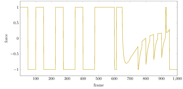
Running the saturating controller (-1 <= F <= 1) from the same initial conditions.

As we can see, our force saturates from the beginning, and is insufficient to stabilize the robot:

We can instead include the saturation constraint in our optimization problem:

\[\begin{matrix}\underset{\boldsymbol{x}}{\text{maximize}} & \sum_{i=1}^N \gamma^{i-1} R(s^{(i)}, a^{(i)}) & \\ \text{subject to} & s^{(i+1)} = T_s s^{(i)} + T_a a^{(i)} & \text{for } i = 1:N \\ & a_\text{min} \leq a^{(i)} \leq a_\text{max} & \text{for } i = 1:N \end{matrix}\]

This problem is significantly more difficult to solve. The added constraints make our problem non-linear, which messes up our previous analysis. Plus, our optimal policy now depends on the initial state.

The problem is still convex though, so we can just throw it into a convex solver and get a solution.

N = 200
a = Convex.Variable(N)
s = Convex.Variable(4, N+1)
problem = maximize(sum(γ^(i-1)*(quadform(s[:,i], Rs) + quadform(a[i], Ra)) for i in 1:N))
problem.constraints += s[:,1] == s₁
for i in 1:N
    problem.constraints += s[:,i+1] == Ts*s[:,i] + Ta*a[i]
    problem.constraints += a_min <= a[i]
    problem.constraints += a[i] <= a_max
end
optimizer = ECOS.Optimizer()
solve!(problem, optimizer)

Solving to 200 steps from the same initial state gives us:

Yellow is the original policy, red is the optimized policy

Unfortunately, the gif above shows the optimized trajectory. That’s different than the actual trajectory we get when we use the nonlinear dynamics. There, Little Tippy tips over:

What we really should be doing is re-solve our policy at every time step. Implementing this on a real robot requires getting it to run faster than 50Hz, which shouldn’t be a problem.

Unfortunately, if we implement that, we can’t quite stabilize:

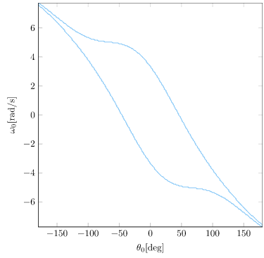
As it turns out, there are states from which Little Tippy, with limited actuation power, does not stabilize with an LQR policy. We can plot the states in which the original LQR policy with infinite actuation stabilizes from \(x = v = 0\) (and does not exceed the \(x\) bounds):

All states in the center between the blue contour lines are initial states within which the cart-pole will reach the stable target state (and not exceed the position boundaries).

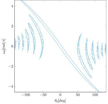
We can produce the same plot for the same LQR policy run with limited actuation:

States within a blue region are initial states from which the LQR policy, when run with clamped outputs, reaches the stable target state.

We can see how severe the actuator limits are! To get our robot to really work, we’re going to want to be able to operate despite these actuator limitations. We’re not going to want to assume that we start from somewhere feasible – we’ll want Little Tipple to know how to build up the momentum necessary to swing up the pole and stabilize.

A Cart Pole Search Problem

There are multiple ways that we can get Little Tippy to swing up. We could try something like iLQR, but that won’t necessarily save us from the nonlinear troughs that are the cart-pole problem. It follows a descent direction just like LQR, so unless our problem is convex or we get lucky, we’ll end up in a mere local minimum.

To help Little Tippy find his way to equilibrium, we’ll do something more basic – transform the problem into a search problem. Up until this point, we’ve been using continuous controls techniques to find optimal control sequences. These are excellent for local refinement. Instead, we need to branch out and consider multiple options, and choose between them for the best path to our goal.

We only need a few things to define a search problem:

  • A state space \(\mathcal{S}\), which defines the possible system configurations
  • An action space \(\mathcal{A}\), which defines the actions available to us
  • A deterministic transition function \(T(s,a)\) that applies an action to a state and produces a successor state
  • A reward function \(R(s,a)\) that judges a state and the taken action for goodness (higher values are better)

Many search problems additionally define some sort of is_done method that checks whether we are in a terminal (ex: goal) state. For example, in the cart-pole problem, we terminate if Little Tippy deviates too far left or right. We could technically incorporate is_done into our reward, by assigning zero reward whenever we match its conditions, but algorithms like forward search can save some compute by explicitly using it.

The cart-pole problem that we have been solving is already a search problem. We have:

  • A state space \(\mathcal{S} = \mathbb{R}^4\) that consists of cart-pole states
  • An action space \(\mathcal{A} = \{ a \in \mathbb{R}^1 | a \in [-1,1]\}\) of bounded, continuous force values
  • A transition function \(T(s,a)\) that takes a cart-pole state and propagates it with the instantaneous state derivative for \(\Delta t\) to obtain the successor state \(s’\)
  • A reward function that, so far, we’ve defined as quadratic in order to apply the LQR machinery, \(R(s,a) = s^\top R_s s + a^\top R_a a\)

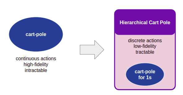
Unfortunately, this search problem is made difficult by the fact that it both has an infinite number of actions (since our actions are continuous) and has very long trajectories, as \(\Delta t = 0.02\). Searching for good paths would be pretty difficult. So, what I am going to try is to create a simpler search problem that acts as a higher-level, coarser problem representation, but is powerful enough to let us find our way to our destination.

Let’s create a new problem. We’ll call it Hierarchical Cart Pole. The states in this problem are cart-pole states, but the actions are to apply an LQR controller for 1 second. We will create a number of LQR controllers, each for the cart-pole problem linearized around different control points. This gives us the nice smooth control capabilities of an LQR controller, but in a search problem that we can actually do things with.

We have:

  • A state space \(\mathcal{S} = \mathbb{R}^4\) that consists of cart-pole states
  • An action space \(\mathcal{A} = \left\{a_1, a_2, \ldots, a_K \right\}\) that consists of choosing between \(K\) controllers
  • A transition function \(T(s,a)\) that takes a cart-pole state and propagates it using the selected LQR controller for 1s
  • A reward function:
    \[R(s,a) = \begin{cases} \frac{1}{100}r_x + r_\theta & \text{if } x \in [-x_\text{min}, x_\text{max}] \\ 0 & \text{otherwise}\end{cases}\]

The reward function simply gives zero reward for out-of-bounds carts, and otherwise produces more reward the closer Little Tipple is to our target state (\(x = 0, \theta = 0\)). I used \(x_\text{max} = -x_\text{min} = 4.8\) just like the original formulation, \(r_x = x_\text{max}^2 – x^2\), and \(r_\theta = 1 + \cos \theta\).

We can now apply any search algorithm to our Hierarchical Cart Pole problem. I used a simple forward search that tries all possible 4-step action sequences. That is enough to give us pretty nice results:

Starting from rest, Little Tippy builds up momentum and swings up the pole!

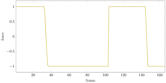
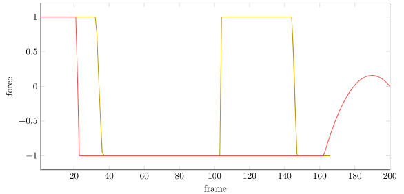
We can plot the forces:

The forces are nice and bounded. We can see the quintessential riding of the rails, with the force bouncing back and forth between its limits. This is quite natural. If we have limits, we’re often going to use everything available to us to get the job done.

In this problem, I linearized the dynamics around 12 control states, all with \(v = \omega = 0\):

reference_states = [
    CartPoleState(-1.0, 0.0, 0.0, 0.0),
    CartPoleState( 0.0, 0.0, 0.0, 0.0),
    CartPoleState( 1.0, 0.0, 0.0, 0.0),
    CartPoleState(-1.0, 0.0, deg2rad(-90), 0.0),
    CartPoleState( 0.0, 0.0, deg2rad(-90), 0.0),
    CartPoleState( 1.0, 0.0, deg2rad(-90), 0.0),
    CartPoleState(-1.0, 0.0, deg2rad(90), 0.0),
    CartPoleState( 0.0, 0.0, deg2rad(90), 0.0),
    CartPoleState( 1.0, 0.0, deg2rad(90), 0.0),
    CartPoleState(-1.0, 0.0, deg2rad(180), 0.0),
    CartPoleState( 0.0, 0.0, deg2rad(180), 0.0),
    CartPoleState( 1.0, 0.0, deg2rad(180), 0.0),
]

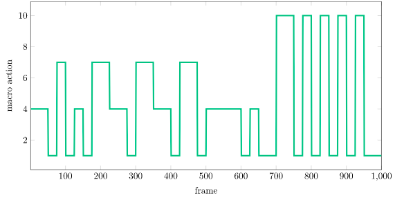
We can plot the macro actions as well, which at each time step is the index of the selected reference state:

Notice how, at the end, the system chooses 1, which is the LQR controller linearized about \(x = -1\). This is what gets the cart to drive left while remaining stabilized.

Linearization

Alright, I know what you’re thinking. Sweet little solver, but how did you get those LQR controllers?

Before we merely linearized about zero. Now we’re linearizing about other control points.

To do this, we start by linearizing our equations of motion. This means we’re forming the 1st order Taylor approximation. The first-order Taylor approximation of some function \(g(x)\) about a reference \(x_\text{ref}\) is \(g(x) \approx g(x_\text{ref}) + g'(x_\text{ref}) (x – x_\text{ref})\). If the equations of motion are \( \dot{s} = F(s, a)\), then the 1st order Taylor approximation about a reference state \(s_\text{ref}\) and a reference action \(a_\text{ref}\) is

\[\dot{s} \approx F(s_\text{ref}, a_\text{ref}) + J_s \cdot (s – s_\text{ref}) + J_a \cdot (a – a_\text{ref})\]

where \(J_s\) and \(J_a\) are the state and action Jacobians (matrices of gradients). Here I always used a reference action of zero.

Why compute this by hand when you could have the computer do it for you? This is what auto-differentiating packages like Zygote.jl are for. I ended up using Symbolics.jl so I could see the symbolic output:

function linearize(mdp::CartPole, s_ref::CartPoleState)
    Δt = mdp.Δt
    @variables x v θ ω ℓ g m M F
    η = (F + m**sin(θ)*ω^2) / M
    pole_α = simplify((M*g*sin(θ) - M*η*cos(θ))/(*(4//3*M - m*cos(θ)^2)))
    cart_a = simplify(η - m ** pole_α * cos(θ) / M)
    # Our first order derivatives
    equations_of_motion = [
        v,
        cart_a,
        ω,
        pole_α
    ]
    state_vars = [x,v,θ,ω]
    action_vars = [F]
    ns = length(state_vars)
    na = length(action_vars)
    df = Array{Float64}(undef, ns)
    Js = Array{Float64}(undef, ns, ns)
    Ja = Array{Float64}(undef, ns, na)
    subs = Dict(x => s_ref.x, v => s_ref.v, θ => s_ref.θ, ω => s_ref.ω,
                m => mdp.mass_pole, M => mdp.mass_pole + mdp.mass_cart,
                g => mdp.gravity, ℓ => mdp.pole_length, F => 0.0)
    for (i, eom) in enumerate(equations_of_motion)
        df[i] = value.(substitute.(eom, (subs,))[1])
        for (j, var) in enumerate(state_vars)
            derivative = expand_derivatives(Differential(var)(eom))
            Js[i,j] = value.(substitute.(derivative, (subs,))[1])
        end
        for (j, var) in enumerate(action_vars)
            derivative = expand_derivatives(Differential(var)(eom))
            Ja[i,j] = value.(substitute.(derivative, (subs,))[1])
        end
    end
    return (df, Js, Ja)
end

The intermediate system, before the reference state is substituted in, is:

\[\begin{bmatrix} \dot{x} \\ \dot{v} \\ \dot{\theta} \\ \dot{\omega} \end{bmatrix} \approx \left. \begin{bmatrix} v \\ \zeta – \frac{m_p \ell \ddot{\theta} \cos(\theta)}{m_p + m_c} \\ \omega \\ \frac{g\sin(\theta) – \zeta \cos(\theta)}{\ell\left( \frac{4}{3} – \frac{m_p \cos(\theta)^2}{m_p + m_c} \right)} \end{bmatrix} \right|_{s = s_\text{ref}} + \left. \begin{bmatrix} 0 & 1 & 0 & 0 \\ 0 & 0 & \frac{-m_p g}{\frac{4}{3}M – m_p} & \frac{\partial}{\partial \omega} \ddot{x} \\ 0 & 0 & 0 & 1 \\ 0 & 0 & \frac{Mg}{\ell \left(\frac{4}{3}M – m_p\right)} & \frac{-m_p \omega \sin (2 \theta)}{\frac{4}{3}M – m_p \cos^2 (\theta)} \end{bmatrix}\right|_{s = s_\text{ref}} \begin{bmatrix} x \\ v \\ \theta \\ \omega \end{bmatrix} + \left. \begin{bmatrix} 0 \\ \frac{\frac{4}{3}}{\frac{4}{3}M – m_p} \\ 0 \\ -\frac{1}{\ell\left(\frac{4}{3}M – m_p\right)}\end{bmatrix}\right|_{s = s_\text{ref}} a\]

where \(\ell\) is the length of the pole, \(m_p\) is the mass of the pole, \(M = m_p + m_c\) is the total mass of the cart-pole system,

\[\zeta = \frac{a + m_p \ell \sin(\theta) \omega^2}{m_p + m_c}\text{,}\]

and

\[\frac{\partial}{\partial \omega} \ddot{x} = m_p \omega \ell \frac{m_p \cos (\theta)\sin(2\theta) – 2 m_p\cos^2(\theta) \sin (\theta) + \frac{8}{3}M \sin(\theta)}{M\left(\frac{4}{3}M – m_p\cos^2(\theta)\right)}\]

For example, linearizing around \(s_\text{ref} = [1.0, 0.3, 0.5, 0.7]\) gives us:

\[\begin{bmatrix} \dot{x} \\ \dot{v} \\ \dot{\theta} \\ \dot{\omega} \end{bmatrix} \approx \begin{bmatrix} \hphantom{-}0.300 \\ -0.274 \\ \hphantom{-}0.700 \\ \hphantom{-}3.704 \end{bmatrix} + \begin{bmatrix} 0 & 1 & 0 & 0 \\ 0 & 0 & -0.323 & 0.064 \\ 0 & 0 & 0 & 1 \\ 0 & 0 & 6.564 & -0.042 \end{bmatrix} \begin{bmatrix} x \\ v \\ \theta \\ \omega \end{bmatrix} + \begin{bmatrix} 0 \\ \hphantom{-}0.959 \\ 0 \\ -0.632\end{bmatrix} a\]

We’re not quite done yet. We want to get our equations into the form of linear dynamics, \(s’ = T_s s + T_a a\). Just as before, we apply Euler integration to our linearized equations of motion:

\[\begin{aligned}s’ & \approx s + \Delta t \dot{s} \\ &= s + \Delta t \left( F(s_\text{ref}, a_\text{ref}) + J_s \cdot (s – s_\text{ref}) + J_a a \right) \\ &= s + \Delta t F(s_\text{ref}, a_\text{ref}) + \Delta t J_s s – \Delta t J_s s_\text{ref} + \Delta t J_a a \\ &= \left(I + \Delta t J_s \right) s + \left( \Delta t F(s_\text{ref}, a_\text{ref}) – \Delta t J_s s_\text{ref} \right) + \Delta t J_a a \end{aligned}\]

So, to get it in the form we want, we have to introduce a 5th state that is always 1. This gives us the linear dynamics we want:

\[\begin{bmatrix} s \\ 1 \end{bmatrix} \approx \begin{bmatrix} I + \Delta t J_s & \Delta t F(s_\text{ref}, a_\text{ref}) – \Delta t J_s s_\text{ref} \\ [0\>0\>0\>0] & 1 \end{bmatrix} \begin{bmatrix} s \\ 1\end{bmatrix} + \begin{bmatrix} \Delta t J_a \\ 0 \end{bmatrix} a\]

For the example reference state above, we get:

\[\begin{bmatrix}x’ \\ v’ \\ \theta’ \\ \omega’ \\ 1\end{bmatrix} \approx \begin{bmatrix}1 & 0.02 & 0 & 0 & 0 \\ 0 & 1 & -0.00646 & 0.00129 & -0.00315 \\ 0 & 0 & 1 & 0.02 & 0 \\ 0 & 0 & 0.131 & 0.999 & 0.00903 \\ 0 & 0 & 0 & 0 & 1\end{bmatrix}\begin{bmatrix}x \\ v \\ \theta \\ \omega \\ 1\end{bmatrix} + \begin{bmatrix}0 \\ 0.019 \\ 0 \\ -0.0126 \\ 0\end{bmatrix}\]

We can take our new \(T_s\) and \(T_a\), slap an extra dimension onto our previous \(R_s\), and use the same LQR machinery as in the previous post to come up with a controller. This gives us a new control matrix \(K\), which we use as a policy:

\[\pi(s) = K \begin{bmatrix}x – x_\text{ref} \\ v – v_\text{ref} \\ \text{angle_dist}(\theta, \theta_\text{ref}) \\ \omega – \omega_\text{ref} \\ 1\end{bmatrix}\]

For our running example, \(K = [2.080, 3.971, 44.59, 17.50, 2.589]\). Notice how the extra dimension formulation can give us a constant force component.

The policy above was derived with the \(R_s\) from the previous post, diagm([-5, -1, -5, -1]). As an aside, we can play around with it to get some other neat control strategies. For example, we can set the first element to zero if we want to ignore \(x\) and control about velocity. Below is a controller that tries to balance the pole while maintaining \(v = 1\):

That is how you might develop a controller for, say, an RC car that you want to stay stable around an input forward speed.

Conclusion

In this post we helped out Little Tippy further by coming up with a control strategy by which he could get to stability despite having actuator limits. We showed that it could (partially) be done by explicitly incorporating the limits into the linearized optimization problem, but that this was limited to the small local domain around the control point. For larger deviations we used a higher-level policy that selected between multiple LQR strategies to search for the most promising path to stability.

I want to stress that the forward search strategy used isn’t world-class by any stretch of the imagination. It does, however, exemplify the concept of tackling a high-resolution problem that we want to solve over an incredibly long time horizon (cart-pole swingup) with a hierarchical approach. We use LQR theory for what it does best – optimal control around a reference point – and build a coarser problem around it that uses said controllers to achieve our goals.

The code for this little project is available here.

Cart Pole Controllers

Here we have a sad little cart-pole robot:

The cart-pole robot is sad because it can’t balance its pole. The poor thing is struggling. Look at it, just floundering around.

Let’s help it out.

Linear Control Theory

Ideally we’d just tell the robot how to balance its pole, but unfortunately we don’t exactly know how to do that. Sure – once the pole is up you kind of want to shift back and forth to counteract its sway, but that only works once its mostly balanced. Getting it up there requires other behavior. Seems kind of complicated.

But fear not! We can break out control theory and then construct a controller.

Let’s see. Okay, we start with the nonlinear dynamics given by Open AI’s cart-pole problem. Our state is given by a position \(x\), a speed \(v\), an angle from vertical \(\theta\) (in radians) and an angular speed \(\omega\). The cart has mass \(m_c\), the pole has mass \(m_p\) and the pole has length \(\ell\). The robot can use its wheels to exert a lateral force \(F\). Our transition dynamics are:

\[\zeta = \frac{F + m_p \ell \sin(\theta) \omega^2}{m_p + m_c}\]

\[\ddot{\theta} = \frac{g\sin(\theta) – \zeta \cos(\theta)}{\ell\left( \frac{4}{3} – \frac{m_p \cos(\theta)^2}{m_p + m_c} \right)}\]

\[\ddot{x} = \zeta – \frac{m_p \ell \ddot{\theta} \cos(\theta)}{m_p + m_c}\]

Once we compute these values, we can thus use Euler integration to update our state by a small timestep \(\Delta t\):

\[ \begin{bmatrix} x’ \\ v’ \\ \theta’ \\ \omega’ \end{bmatrix} = \begin{bmatrix} x \\ v \\ \theta \\ \omega \end{bmatrix} + \Delta t \begin{bmatrix} v \\ \ddot{x} \\ \omega \\ \ddot{\theta} \end{bmatrix} \]

Linear control theory requires that our dynamics be linear. As such, we linearize our system about our target stable point (\(x = v = \theta = \omega = 0\)) by computing the Jacobian and forming a linear system:

\[\begin{bmatrix} \dot{x} \\ \dot{v} \\ \dot{\theta} \\ \dot{\omega} \end{bmatrix} \approx \begin{bmatrix} \frac{\partial}{\partial x} v & \frac{\partial}{\partial v} v & \frac{\partial}{\partial \theta} v & \frac{\partial}{\partial \omega} v \\ \frac{\partial}{\partial x} \ddot{x} & \frac{\partial}{\partial v} \ddot{x} & \frac{\partial}{\partial \theta} \ddot{x} & \frac{\partial}{\partial \omega} \ddot{x} \\ \frac{\partial}{\partial x} \omega & \frac{\partial}{\partial v} \omega & \frac{\partial}{\partial \theta} \omega & \frac{\partial}{\partial \omega} \omega \\ \frac{\partial}{\partial x} \ddot{\theta} & \frac{\partial}{\partial v} \ddot{\theta} & \frac{\partial}{\partial \theta} \ddot{\theta} & \frac{\partial}{\partial \omega} \ddot{\theta} \end{bmatrix} \begin{bmatrix} x \\ v \\ \theta \\ \omega \end{bmatrix} + \begin{bmatrix} \frac{\partial}{\partial F} v \\ \frac{\partial}{\partial F} \ddot{x} \\ \frac{\partial}{\partial F} \omega \\ \frac{\partial}{\partial F} \ddot{\theta} \end{bmatrix} F \]

I used Symbolics.jl to do the heavy lifting for me, which resulted in:

\[\begin{bmatrix} \dot{x} \\ \dot{v} \\ \dot{\theta} \\ \dot{\omega} \end{bmatrix} \approx \begin{bmatrix} 0 & 1 & 0 & 0 \\ 0 & 0 & \frac{-m_p g}{\frac{4}{3}M – m_p} & 0 \\ 0 & 0 & 0 & 1 \\ 0 & 0 & \frac{Mg}{\ell \left(\frac{4}{3}M – m_p\right)} & 0 \end{bmatrix} \begin{bmatrix} x \\ v \\ \theta \\ \omega \end{bmatrix} + \begin{bmatrix} 0 \\ \frac{\frac{4}{3}}{\frac{4}{3}M – m_p} \\ 0 \\ -\frac{1}{\ell\left(\frac{4}{3}M – m_p\right)}\end{bmatrix} F\]

where \(M = m_p + m_c\).

We can produce a linear controller \(F = K s\) for our linear system. In this case, \(K\) is simply a vector that determines the feedback gains for each of the state components.

I am using a basic cart pole environment, with \(\Delta t = 0.02, m_c = 1, m_p = 0.1, g = 9.8\). After some experimentation, \(K = [1.0, -0.5, 100.0, 1.0]\) worked pretty well. Here is how the little cart-pole guys is doing with that:

Much better! We’ve got the little guy balancing around his stable point. As long as he starts relatively close to stability, he’ll pop right back. And we did it with some math and tuning.

Automatic Tuning

Unfortunately, our gain matrix \(K\) sort of came out of nowhere. Ideally there would be a better way to derive one.

Fortunately for us, there is. We are going to derive the gain matrix using the optimal policy for linear quadratic regulator (LQR) problems. (These are covered in section 7.8 of Alg4DM.)

An LQR problem has linear dynamics:

\[s^{(k+1)} = T_s s^{(k)} + T_a a^{(k)} + w\]

where \(T_s\) and \(T_a\) are matrices, \(s\) is our state, \(a\) is our action, and \(w\) is zero-mean noise.

We already have the equation \(s^{(k+1)} = s^{(k)} + \dot{s}^{(k)} \Delta t\), and can get our linear dynamics that way:

\[\begin{bmatrix} x \\ v \\ \theta \\ \omega \end{bmatrix}^{(k+1)} = \begin{bmatrix} x \\ v \\ \theta \\ \omega \end{bmatrix}^{(k)} + \left(\begin{bmatrix} 0 & 1 & 0 & 0 \\ 0 & 0 & \frac{-m_p g}{\frac{4}{3}M – m_p} & 0 \\ 0 & 0 & 0 & 1 \\ 0 & 0 & \frac{Mg}{\ell \left(\frac{4}{3}M – m_p\right)} & 0 \end{bmatrix} \begin{bmatrix} x \\ v \\ \theta \\ \omega \end{bmatrix}^{(k)} + \begin{bmatrix} 0 \\ \frac{\frac{4}{3}}{\frac{4}{3}M – m_p} \\ 0 \\ -\frac{1}{\ell\left(\frac{4}{3}M – m_p\right)}\end{bmatrix} F^{(k)}\right) \Delta t + w\]

which simplifies to:

\[\begin{bmatrix} x \\ v \\ \theta \\ \omega \end{bmatrix}^{(k+1)} = \begin{bmatrix} 1 & \Delta t & 0 & 0 \\ 0 & 1 & \frac{-m_p g \Delta t}{\frac{4}{3}M – m_p} & 0 \\ 0 & 0 & 1 & \Delta t \\ 0 & 0 & \frac{M g \Delta t}{\ell \left(\frac{4}{3}M – m_p\right)} & 1 \end{bmatrix} \begin{bmatrix} x \\ v \\ \theta \\ \omega \end{bmatrix}^{(k)} + \begin{bmatrix} 0 \\ \frac{\frac{4}{3} \Delta t}{\frac{4}{3}M – m_p} \\ 0 \\ -\frac{\Delta t}{\ell\left(\frac{4}{3}M – m_p\right)}\end{bmatrix} F^{(k)} + w\]

An LQR problem additionally has quadratic rewards:

\[R(s,a) = s^\top R_s s + a^\top R_a a\]

which is accumulated across all timesteps.

As engineers, we get to choose the reward function that best captures quality in our problem, and then the LQR machinery will produce an optimal policy with respect to that reward function. Note that the LQR process only works if \(R_s\) and \(R_a\) overall produce costs, which amounts to \(R_s\) being negative semidefinite and \(R_a\) being negative definite.

Let’s simply penalize deviations from zero, with more weight given to the linear and angular positions:

\[R_s = \begin{bmatrix} -5 & 0 & 0 & 0 \\ 0 & -1 & 0 & 0 \\ 0 & 0 & -5 & 0 \\ 0 & 0 & 0 & -1 \end{bmatrix} \qquad R_s = \begin{bmatrix} -1 \end{bmatrix}\]

and the value of \(R_s\) determines how much to penalize large magnitudes of force.

If we plug these into an LQR solver, crank up the horizon, and pick the maximum-horizon control matrix, we get \(K = [2.06942, 3.84145, 43.32, 15.745]\). And if we load that up into our little robot, we get:

Wow! That’s pretty darn stable.

Let’s show it with a more adverse starting state:

Very cool.

Conclusion

To recap, we’ve just used LQR theory to derive our controller rather than just hand tune one. We got something procedural that works a lot better than what I got by hand. (I even got the sign on velocity wrong in my original gain matrix). Notice that we still had to specify something by hand, namely the rewards, but they were much easier to specify to still get something good.

This concludes this blog post, but it doesn’t conclude our cart-pole shenanigans. We’ve helped Tippy the Robot, but only with control theory. What if we don’t have continuous force output? What if we don’t have an unbounded output force? What if we want to be able to swing up from bad starting states? What if we don’t know the equations of motion? We’ll take a stab at it next time.

Convex Duality

Convex duality is the sort of thing where you see the symbolic derivation and it sort of makes sense, but then you forget the steps and a day or two later you just sort of have to trust yourself that the theorems and facts hold but forget where they really come from. I recently relearned convex duality from the great lectures of Stephen Boyd, and in so doing, also learned about a neat geometry interpretation that helps solidify things.

Working with Infinite Steps

Everything starts with an optimization problem in standard form:

\[\begin{matrix}\underset{\boldsymbol{x}}{\text{minimize}} & f(\boldsymbol{x}) \\ \text{subject to} & \boldsymbol{g}(\boldsymbol{x}) \leq \boldsymbol{0} \\ & \boldsymbol{h}(\boldsymbol{x}) = \boldsymbol{0} \end{matrix}\]

This problem has an objective \(f(\boldsymbol{x})\), some number of inequality constraints \(\boldsymbol{g}(\boldsymbol{x}) \leq \boldsymbol{0}\), and some number of equality constraints \(\boldsymbol{h}(\boldsymbol{x}) = \boldsymbol{0}\).

Solving an unconstrained optimization problem often involves sampling the objective and using its gradient, or several local values, to know which direction to head in to find a better design \(\boldsymbol{x}\). Solving a constrained optimization problem isn’t as straightforward – we cannot accept a design that violates any constraints.

We can, however, view our constrained optimization problem as an unconstrained optimization problem. We simply incorporate our constraints into our objective, setting them to infinity when the constraints are violated and setting them to zero when the constraints are met:

\[\underset{\boldsymbol{x}}{\text{minimize}} \enspace f(\boldsymbol{x}) + \sum_i \infty \cdot \left( g_i(\boldsymbol{x}) > 0\right) + \sum_j \infty \cdot \left( h_j(\boldsymbol{x}) \neq 0\right)\]

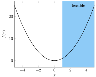
For example, if our problem is

\[\begin{matrix}\underset{x}{\text{minimize}} & x^2 \\ \text{subject to} & x \geq 1 \end{matrix}\]

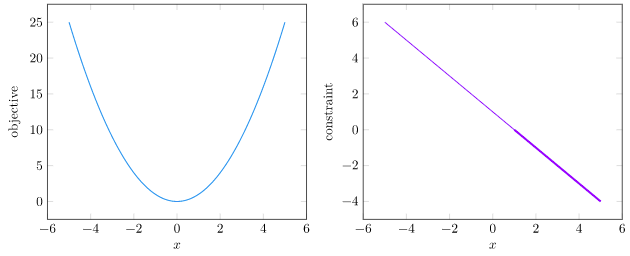
which looks like this

then we can rewrite it as

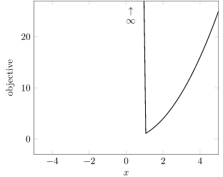
\[\underset{x}{\text{minimize}} \enspace x^2+\infty \cdot \left( x < 1\right)\]

which looks like

We’ve simply raised the value of infeasible points to infinity. Problem solved?

By doing this, we made our optimization problem much harder to solve with local methods. The gradient of designs in the infeasible region is zero, so we cannot use those to know which way to progress toward feasibility. It is also discontinuous. Furthermore, infinity is rather difficult to work with – it just produces more infinities when added or multiplied to most numbers. This new optimization problem is perhaps simpler, but we’ve lost a lot of information.

What we can do instead is reinterpret our objective slightly. What if, instead of using this infinite step, we simply multiplied our inequality function \(g(x) = 1 – x\) by a scalar \(\lambda\)?

\[\underset{x}{\text{minimize}} \enspace x^2+ \lambda \left( 1 – x \right)\]

If we have a feasible \(x\), then \(\lambda = 0\) gives us the original objective function. If we have an infeasible \(x\), then \(\lambda = \infty\) gives us the penalized objective function.

We’re taking the objective and constraint, which are separate functions:

and combining them into a single objective based on \(\lambda\):

Let’s call our modified objective function the Lagrangian:

\[\mathcal{L}(x, \lambda) = x^2+ \lambda \left( 1 – x \right)\]

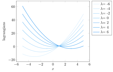
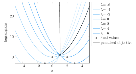
If we fix \(\lambda\), we can minimize our objective over \(x\). I am going to call these dual values:

We find that all of these dual values are below the optimal value of the original problem:

This in itself is a big deal. We can produce a lower bound on the optimal value simply by minimizing the Lagrangian. Why is this?

Well, it turns out that we are guaranteed to get a lower bound any time that \(\lambda \geq 0\). This is because a positive \(\lambda\) ensures that our penalized objective is at or below the original objective for all feasible points. Minimizing is thus guaranteed to give us a design at or below the original value.

This is such a big deal, that we’ll call this minimization problem the Lagrange dual function, and give it a shorthand:

\[\mathcal{D}(\lambda) = \underset{x}{\text{minimize}} \enspace \mathcal{L}(x, \lambda)\]

which for our problem is

\[\mathcal{D}(\lambda) = \underset{x}{\text{minimize}} \enspace x^2 + \lambda \left( 1 – x \right)\]

Okay, so we have a way to get a lower bound. How about we get the *best* lower bound? That gives rise to the Lagrange dual problem:

\[\underset{\lambda \geq 0}{\text{maximize}} \enspace \mathcal{D}(\lambda)\]

For our example problem, the best lower bound is given by \(\lambda = 2\), which produces \(x = 1\), \(f(x) = 1\). This is the solution to the original problem.

Having access to a lower bound can be incredibly useful. It isn’t guaranteed to be useful (the lower bound can be \(-\infty\)), but it can also be relatively close to optimal. For convex problems, the bound is tight – the solution to the Lagrange dual problem has the same value as the solution to the original (primal) problem.

A Geometric Interpretation

We’ve been working with a lot of symbols. We have some plots, but I’d love to build further intuition with a geometric interpretation. This interpretation also comes from Boyd’s lectures, and textbook.

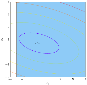
Let’s work with a slightly beefier optimization problem with a single inequality constraint:

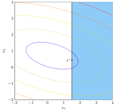
\[\begin{matrix}\underset{\boldsymbol{x}}{\text{minimize}} & \|\boldsymbol{A} \boldsymbol{x} – \boldsymbol{b} \|_2^2 \\ \text{subject to} & x_1 \geq c \end{matrix}\]

In this case, I’ll use

\[\boldsymbol{A} = \begin{bmatrix} 1 & 0.3 \\ 0.3 & 2\end{bmatrix} \qquad \boldsymbol{b} = \begin{bmatrix} 0.5 \\ 1.5\end{bmatrix} \qquad c = 1.5\]

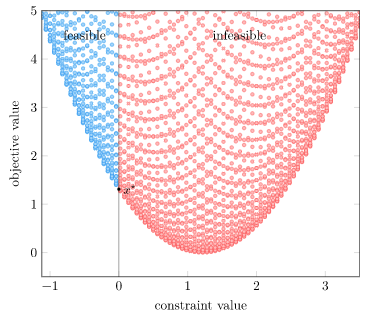
Let’s plot the objective, show the feasible set in blue, and show the optimal solution:

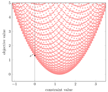
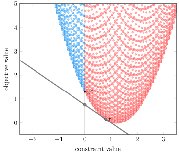
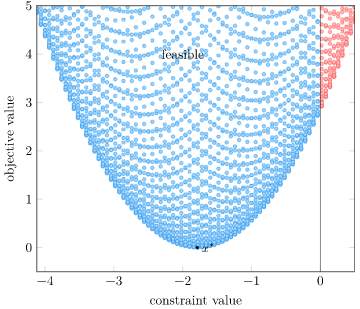
Our Lagrangian is again comprised of two terms – the objective function \( \|\boldsymbol{A} \boldsymbol{x} – \boldsymbol{b} \|_2^2\) and the constraint \(\lambda (c – x_1)\). We can build a neat geometric interpretation of convex duality by plotting (constraint, objective) pairs for various values of \(\boldsymbol{x}\):

We get a parabolic region. This isn’t a huge surprise, given that we have a quadratic objective function.

Note that the horizontal axis is the constraint value. We only have feasibility when \(g(\boldsymbol{x}) \leq 0\), so our feasible designs are those left of the vertical line.

I’ve already plotted the optimal value – it is at the bottom of the feasible region. (Lower objective function values are better, and the bottom has the lowest value).
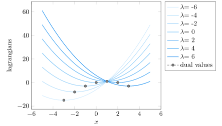
Let’s see if we can include our Lagrangian. The Lagrangian is:

\[\mathcal{L}(\boldsymbol{x}, \lambda) = f(\boldsymbol{x}) + \lambda g(\boldsymbol{x})\]

If we fix \(\boldsymbol{x}\), it is linear!

The Lagrange dual function is

\[\mathcal{D}(\lambda) = \underset{\boldsymbol{x}}{\text{minimize}} \enspace f(\boldsymbol{x}) + \lambda g(\boldsymbol{x})\]

If we evaluate \(\mathcal{D}\) for a particular \(\lambda\), we’ll minimize and get a design \(\hat{\boldsymbol{x}}\). The value of \(\mathcal{D}(\lambda)\) will be \(f(\hat{\boldsymbol{x}}) + \lambda g(\hat{\boldsymbol{x}})\). Remember, for \(\lambda \geq 0\) this is a lower bound. Said lower bound is the y-intercept of the line with slope \(-\lambda\) that passed through our (constraint, objective) at \(\hat{\boldsymbol{x}}\).
For example, with \(\lambda = 0.75\), we get:

We got a lower bound, and it is indeed lower than the true optimum. Furthermore, that line is a supporting hyperplane of our feasible region.

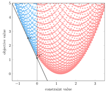
Let’s try it again with \(\lambda = 3\):

Our \(\lambda\) is still non-negative, so we get a valid lower bound. It is below our optimal value.

Now, in solving the Lagrange dual problem we get the best lower bound. This best lower bound just so happens to correspond to the \(\lambda\) that produces a supporting hyperplane at our optimum (\(\lambda \approx 2.15\)):

Our line is tangent at our optimum. This ties in nicely with the KKT conditions (out of scope for this blog post), which require that the gradient of the Lagrangian be zero at the optimum (for a problem with a differentiable objective and constraints), and thus the gradients of the objective and the constraints (weighted by \(\lambda\)) balance out.

Notice that in this case, the inequality constraint was active, with our optimum at the constraint boundary with \(g(\boldsymbol{x}) = 0\). We needed a positive \(\lambda\) to balance against the objective function gradient.

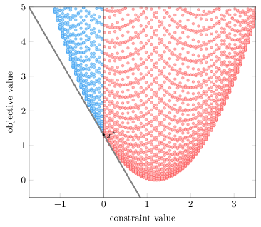
If we change our problem such that the unconstrained optimum is feasible, then we do not need a positive dual value to balance against the objective function gradient. Let’s adjust our constraint to max our solution feasible:

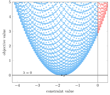
We now get an objective / constraint region with a minimum inside the feasible area:

Our best lower bound is obtained with \(\lambda = 0\):

This demonstrates complementary slackness, the idea that \(\lambda_i g_i(\boldsymbol{x})\) is always zero. If constraint \(i\) is active, \(g_i(\boldsymbol{x}) = 0\);\ and if constraint \(i\) is inactive, \(\lambda_i = 0\).

So with this geometric interpretation, we can think of choosing \(\lambda\) as picking the slope of a line that supports this multidimensional volume from below and to the left. We want the line with the highest y-intercept.

Multiple Constraints (and Equality Constraints)

I started this post off with a problem with multiple inequality and equality constraints. In order to be thorough, I just wanted to mention that the Lagrangian and related concepts extend the way you’d expect:

\[\mathcal{L}(\boldsymbol{x}, \boldsymbol{\lambda}, \boldsymbol{\nu}) = f(\boldsymbol{x}) + \sum_i \lambda_i g_i(\boldsymbol{x}) + \sum_j \nu_j h_j(\boldsymbol{x})\]

and

\[\mathcal{D}(\boldsymbol{\lambda}, \boldsymbol{\nu}) = \underset{\boldsymbol{x}}{\text{maximize}} \enspace \mathcal{L}(\boldsymbol{x}, \boldsymbol{\lambda}, \boldsymbol{\nu})\]

We require that all \(\lambda\) values be nonnegative, but do not need to restrict the \(\nu\) values for the equality constraints. As such, our Lagrangian dual problem is:

\[\underset{\boldsymbol{\lambda} \geq \boldsymbol{0}, \>\boldsymbol{\nu}}{\text{maximize}} \enspace \mathcal{D}(\boldsymbol{\lambda}, \boldsymbol{\nu})\]

The geometric interpretation still holds – it just has more dimensions. We’re just finding supporting hyperplanes.

Embedded Contours with Marching Squares

I recently started working on new chapters for Algorithms for Optimization, starting with a new chapter on quadratic programs. We already have a chapter on linear programs, but quadratic programs are sufficiently different and are ubiquitous enough that giving them their own chapter felt warranted.

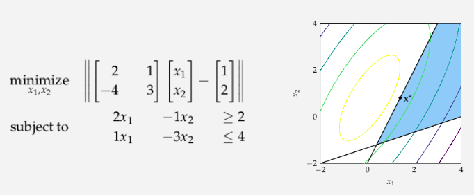
A simple example quadratic program.

The chapter starts with a general formulation for quadratic programs and transforms the problem a few times into simpler and simpler formulations, until we get a nonnegative least squares problem. This can be solved, and then we can use that solution to back our way up the transform stack back to a solution of our original solution.

In texts, these problem transforms are typically solely the realm of mathematical manipulations. While math is of course necessary, I also tried hard to depict what these various problem representations looked like to help build an intuitive understanding of what some of the transformations were. In particular, there was one figure where I wanted to show how the equality constraints of a general-form quadratic program could be removed when formulating a lower-dimensional least squares program:

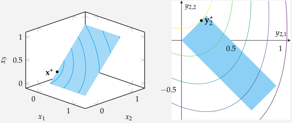
A 3d general-form quadratic program with an equality constraint on the left, and a 2d least squares program on the right.

This post is about this figure, and more specifically, about the blue contour lines on the left side.

What is this Figure?

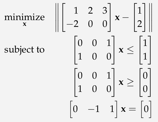
The figure on left shows the following quadratic program:

general-form quadratic program

As we can see, the quadratic program is constrained to lie within a square planar region \(0 \leq x \leq 1\), \(0 \leq x_3 \leq 1\), and \(x_2 = x_3\). The feasible set is shown in blue.

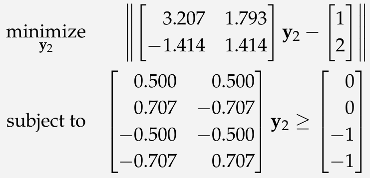
The right figure on the right shows the least-squares program that we get when we factor out the equality constraint. No need to get into the details here, it isn’t really important for this post, but we can use our one equality equation to remove one variable in our original problem, producing a 2d problem without any equality constraints:

least squares program

The original feasible set is rotated and stretched, and the objective function contours are rotated and stretched, but other than that we have a similar topology and a pretty standard problem that we can solve.

How do we Make the Figures?

I make the plots with PGFPlots.jl, which uses the pgfplots LaTeX package under the hood. It is a nice synergy of Julia coding and LaTeX within the LaTeX textbook.

Right Plot

The right plot is pretty straight forward. It has a contour plot for the objective function:

Plots.Contour(x -> norm(A_lsi*x - b_lsi, 2),
              xdomain, ydomain, xbins=600, ybins=600)

some over + under line plots and a fill-between for the feasible region:

x1_domain_feasible = (0.0, (0.5+√2)/2)
push!(plots,
      Plots.Linear(x1->max(-x1, x1 - sqrt(2)), x1_domain_feasible,
                   style="name path=A, draw=none, mark=none"))
push!(plots,
      Plots.Linear(x1->min(x1, 1/2-x1), x1_domain_feasible,
                   style="name path=B, draw=none, mark=none"))
push!(plots,
      Plots.Command("\\addplot[pastelBlue!50] fill between[of=A and B]"))

and a single-point scatter plot plus a label for the solution:

push!(plots,
      Plots.Scatter([x_val[1]], [x_val[2]],
      style="mark=*, mark size=1.25, mark options={solid, draw=black, fill=black}"))
push!(plots,
      Plots.Command("\\node at (axis cs:$(x_val[1]),$(x_val[2])) [anchor=west] {\\small \\textcolor{black}{\$y_2^\\star\$}}"))

These plots get added to an Axis and we’ve got our plot.

Left Plot

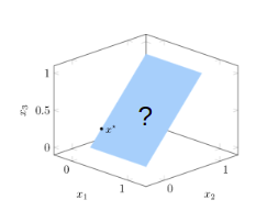
The left plot is in 3D. If we do away with the blue contour lines, its actually even simpler than the right plot. We simply have a square patch, a single-point scatter plot, and our label:

Axis([
   Plots.Command("\\addplot3[patch,patch type=rectangle, faceted color=none, color=pastelBlue!40] coordinates {(0,0,0) (1,0,0) (1,1,1) (0,1,1)}"),
   Plots.Linear3([x_val[1]], [x_val[2]], [x_val[3]], mark="*", style="mark size=1.1, only marks, mark options={draw=black, fill=black}"),
   Plots.Command("\\node at (axis cs:$(x_val[1]),$(x_val[2]),$(x_val[3])) [anchor=west] {\\small \\textcolor{black}{\$x^\\star\$}}"),
  ], 
  xlabel=L"x_1", ylabel=L"x_2", zlabel=L"x_3", width="1.2*$width", 
  style="view={45}{20}, axis equal",
  legendPos="outer north east"
)

The question is – how do we create that contour plot, and how do we get it to lie on that blue patch?

How do you Draw Contours?

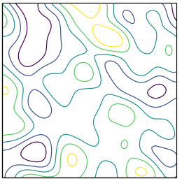
Contour plots don’t seem difficult to plot, until you have to sit down and plot them. They are just lines of constant elevation – in this cases places where \(\|Ax – b\| = c\) for various constants \(c\). But, unlike line plots, where you can just increase \(x\) left to right and plot successive \((x, f(x))\) pairs, for contour plots you don’t know where your line is going to be ahead of time. And that’s assuming you only have one line per contour value – you might have multiple:

A contour plot with multiple contour lines per level.

So, uh, how do we do this?

The first thing I tried was trying to write my function out the traditional way – as \((x_1, f(x_1))\) pairs. Unfortunately, this doesn’t work out, because the contours aren’t 1:1.

The second thing I briefly considered was a search method. If I fix my starting point, say, \(x_1 = 0, x_2 = 0.4\), I can get the contour level \(c = \|Ax – b\| \). Then, I could search toward the right in an arc to find where the next contour line was, maybe bisect over an arc one step distance away and proceed that way:

An iterative search procedure for following a contour line, proceeding left to right.

I think this approach would have worked for this figure, since there were never multiple contour lines for the same contour value, but it would have been more finicky, especially around the boundaries, and it would not have generalized to other figures.

Marching Squares

I happened upon a talk by Casey Muratori on YouTube, “Papers I have Loved“, a few weeks ago. One of the papers Casey talked about was Marching Cubes, A High Resolution 3D Surface Construction Algorithm. This 1987 paper by W. Lorenson and H. Cline presented a very simply way to generate surfaces (in 3D or 2D) in places of constant value: \(f(x) = c\).

Casey talked about it in the context of rendering metaballs, but when I found myself presented with the contour problem, it was clear that marching cubes (or squares, rather, since its 2d) was relevant here too.

The algorithm is a simple idea elegantly applied.

The contour plot we want to make is on a 2d surface in a 3d plot, but let’s just consider the 2d surface for now. Below we show that feasible square along with our objective function, \(f(x) = \|Ax – b\|\):

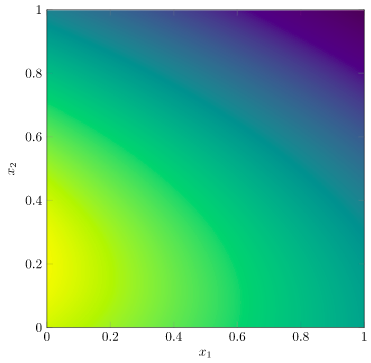
An image plot showing our object function. We want to find contour lines.

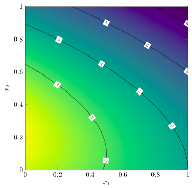
Our objective is to produce contour lines, the same sort as are produced when we make a PGFPlots contour plot:

We already know that there might be multiple connected contour lines for a given level, so a local search method won’t be sufficient. Instead, marching squares uses a global approach combined with local refinement.

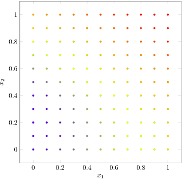
We begin by evaluating a grid of points over our plot:

We’ll start with a small grid, but for higher-quality images we’d make it finer.

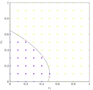
Let’s focus on the contour line \(f(x) = 3\). We now determine, for each vertex in our mesh, whether its value is above or below our contour target of 3. (I’ll plot the contour line too for good measure):

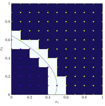
Blue points are where the objective function <= 3, and yellow points are where it is > 3.

Marching squares will now tile the image based on each 4-vertex square, and the binary values we just evaluated. Any squares with all vertices equal can simply be ignored – the contour line doesn’t pass through them. This leaves the following tiles:

The white tiles are those that contain our contour line(s).

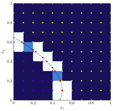
Now, each remaining tile comes in multiple possible “flavors” – the various ways that its vertices can be above or below the objective value. There are \(2^4\) possible tiles, two of which we’ve already discarded, leaving 14 options. The Wikipedia article has a great set of images showing all of the tile combinations, but here we will concern ourselves with two more kinds: tiles with one vertex below or one vertex above, and tiles with two neighboring vertices above and two neighboring vertices below:

The white squares have one vertex above or one vertex below. The gray squares have two neighboring vertices above and two neighboring vertices below.

Let’s start with the first type. These squares have two edges where the function value changes. We know, since we’re assuming our objective function is continuous, that our contour line must pass through those edges. As such, if we run a bisection search along each of those edges, we can quickly identify those crossing points:

The red points are where bisection search has found a crossing point.

We then get our contour plot, for this particular contour value, by drawing all of the line segments between these crossing points:

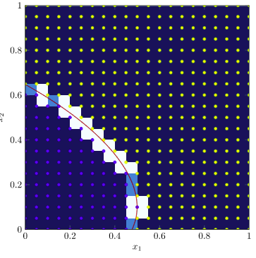
We can get higher resolution contour lines by using a finer grid:

The same contour line with double the resolution.

To get our full contour plot, we simply run marching squares on multiple contour levels. To get the original plot, I run this algorithm to get all of the little tile line segments, then I render them as separate Linear3 line segments on top of the 3d patch. Pretty cool!

The created figure

What does the Code Look Like?

The code for marching squares is pretty elegant.

We start off with defining our grid:

nbins = 41
x1s = collect(range(0.0, stop=1.0, length=nbins))
x2s = collect(range(0.0, stop=1.0, length=nbins))
is_above = falses(length(x1s), length(x2s))

Next we define a bisection method for quickly interpolating between two vertices:

function bisect(
    u_target::Float64, x1_lo::Float64, x1_hi::Float64, 
    x2_lo::Float64, x2_hi::Float64, k_max::Int=8)
    f_lo = norm(A*[x1_lo, x2_lo, x2_lo]-b)
    f_hi = norm(A*[x1_hi, x2_hi, x2_hi]-b)
 
    if f_lo > f_hi # need to swap low and high
        x1_lo, x1_hi, x2_lo, x2_hi = x1_hi, x1_lo, x2_hi, x2_lo
    end
 
    x1_mid = (x1_hi + x1_lo)/2
    x2_mid = (x2_hi + x2_lo)/2
    for k in 1 : k_max
        f_mid = norm(A*[x1_mid, x2_mid, x2_mid] - b)
        if f_mid > u_target
            x1_hi, x2_hi, f_hi = x1_mid, x2_mid, f_mid
        else
            x1_lo, x2_lo, f_lo = x1_mid, x2_mid, f_mid
        end
        x1_mid = (x1_hi + x1_lo)/2
        x2_mid = (x2_hi + x2_lo)/2
    end
 
    return (x1_mid, x2_mid)
end

In this case I’ve baked in the objective function, but you could of course generalize this and pass one in.

We then iterate over our contour levels. For each contour level (u_target), we evaluate the grid and then evaluate all of our square patches and add little segment plots as necessary:

for (i,x1) in enumerate(x1s)
    for (j,x2) in enumerate(x2s)
        is_above[i,j] = norm(A*[x1, x2, x2] - b) > u_target
    end
end
for i in 2:length(x1s)
    for j in 2:length(x2s)
        # bottom-right, bottom-left, top-right, top-left
        bitmask = 0x00
        bitmask |= (is_above[i,j-1] << 3)
        bitmask |= (is_above[i-1,j-1] << 2)
        bitmask |= (is_above[i,j] << 1)
        bitmask |= (is_above[i-1,j])
        plot = true
        x1_lo1 = x1_hi1 = x2_lo1 = x2_hi1 = 0.0
        x1_lo2 = x1_hi2 = x2_lo2 = x2_hi2 = 0.0
        if bitmask == 0b1100 || bitmask == 0b0011
            # horizontal cut
            x1_lo1, x1_hi1, x2_lo1, x2_hi1 = x1s[i-1], x1s[i-1], x2s[j-1], x2s[j]
            x1_lo2, x1_hi2, x2_lo2, x2_hi2 = x1s[i], x1s[i], x2s[j-1], x2s[j]
        elseif bitmask == 0b0101 || bitmask == 0b1010
            # vertical cut
            x1_lo1, x1_hi1, x2_lo1, x2_hi1 = x1s[i-1], x1s[i], x2s[j-1], x2s[j-1]
            x1_lo2, x1_hi2, x2_lo2, x2_hi2 = x1s[i-1], x1s[i], x2s[j], x2s[j]
        elseif bitmask == 0b1000 || bitmask == 0b0111
            # cut across bottom-right
            x1_lo1, x1_hi1, x2_lo1, x2_hi1 = x1s[i-1], x1s[i], x2s[j-1], x2s[j-1]
            x1_lo2, x1_hi2, x2_lo2, x2_hi2 = x1s[i], x1s[i], x2s[j-1], x2s[j]
        elseif bitmask == 0b0100 || bitmask == 0b1011
            # cut across bottom-left
            x1_lo1, x1_hi1, x2_lo1, x2_hi1 = x1s[i-1], x1s[i], x2s[j-1], x2s[j-1]
            x1_lo2, x1_hi2, x2_lo2, x2_hi2 = x1s[i-1], x1s[i-1], x2s[j-1], x2s[j]
        elseif bitmask == 0b0010 || bitmask == 0b1101
            # cut across top-right
            x1_lo1, x1_hi1, x2_lo1, x2_hi1 = x1s[i-1], x1s[i], x2s[j], x2s[j]
            x1_lo2, x1_hi2, x2_lo2, x2_hi2 = x1s[i], x1s[i], x2s[j-1], x2s[j]
        elseif bitmask == 0b0001 || bitmask == 0b1110
            # cut across top-left
            x1_lo1, x1_hi1, x2_lo1, x2_hi1 = x1s[i-1], x1s[i], x2s[j], x2s[j]
            x1_lo2, x1_hi2, x2_lo2, x2_hi2 = x1s[i-1], x1s[i-1], x2s[j-1], x2s[j]
        else
            plot = false
        end
        if plot
            x1a, x2a = bisect(u_target, x1_lo1, x1_hi1, x2_lo1, x2_hi1)
            x1b, x2b = bisect(u_target, x1_lo2, x1_hi2, x2_lo2, x2_hi2)
            push!(contour_segments, 
                Plots.Linear3([x1a, x1b], [x2a, x2b], [x2a, x2b],
                               style="solid, pastelBlue, mark=none")
            )
        end
    end
end

In this code, all we ever do is figure out which two line segments to bisect over, and if we get then, run the bisection and plot the ensuing line. Its actually quite neat and compact.

Conclusion

So there you have it – a home-rolled implementation for contour plotting turns out to be useful for embedding 2d contours in a 3d plot.

Note that the implementation here wasn’t truly general. In this case, we didn’t handle some tile types, namely those where opposing corners have the same aboveness, but neighboring corners have differing aboveness. In those cases, we need to bisect across all four segments, and we typically need to remove ambiguity by sampling in the tile’s center to determine which way the segments cross.

I find it really satisfying to get to apply little bits of knowledge like this from time to time. Its part of computer programming that is endlessly rewarding. I have often been amazed by how a technique that I learned about in one context surprised me by being relevant in something else later on.

Delaunay Triangulations

I recently read a fantastic blog post about Delaunay triangulations and quad-edge data structures, and was inspired to implement the algorithm myself. The post did a very good job of breaking the problem and the algorithm down, and had some really nice interactive elements that made everything make sense. I had tried to grok the quad-edge data structure before, but this was the first time where it really made intuitive sense.

This post covers more or less the same content, in my own words and with my own visualizations. I highly recommend reading the original post.

What is a Delaunay Triangulation

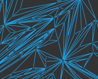
A triangulation is any breakdown of a set of vertices into a set of non-overlapping triangles. Some triangulations are better than others, and the Delaunay triangulation is a triangulation that makes each triangle as equilateral as possible. As a result, it is the triangulation that keeps all of the points in a given triangle as close to each other as possible, which ends up making it quite useful for a lot of spacial operations, such as finite element meshes.

As we can see above, there are a lot of bad triangulations with a lot of skinny triangles. Delaunay triangulations avoid that as much as possible.

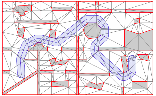
One of the neatest applications of these triangulations is in motion planning. In constrained Delaunay triangulation, you for all walls in your map to be edges in your triangulation, and otherwise construct a normal Delaunay triangulation. Then, your robot can pass through any edge of sufficient length (i.e., if its a wide enough gap), and you can quickly find shortest paths through complicated geometry while avoiding regions you shouldn’t enter:

How to Construct a Delaunay Triangulation

So we want a triangulation that is as equilateral as possible. How, technically, is this achieved?

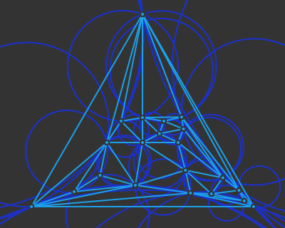
More precisely, a triangulation is Delaunay if no vertex is inside the circumcircle of any of the triangles. (A circumcircle of a triangle is the circle that passes through its three vertices).

The circumcircles for every triangle in a Delaunay triangulation. No circle contains a vertex.

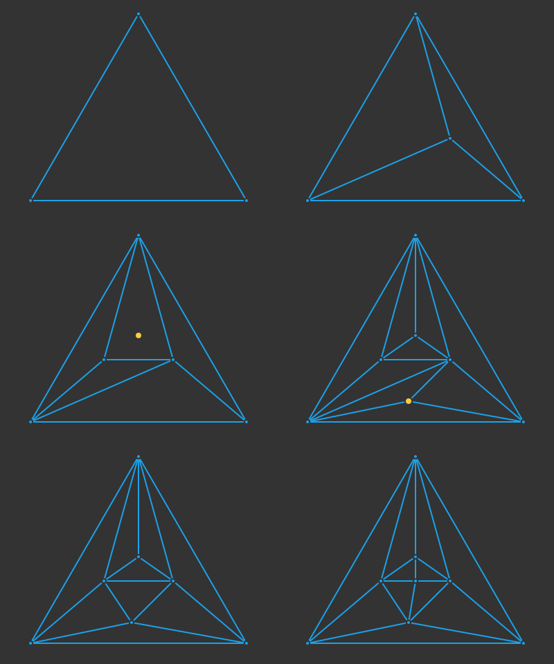
One way to construct a Delaunay triangulation for a set of points is construct one iteratively. The Guibas & Stolfi incremental triangulation algorithm starts with a valid triangulation and repeatedly adds a new point, joining it into the triangulation and then changing edges to ensure that the mesh continues to be a Delaunay triangulation:

Iterative construction of a Delaunay triangulation

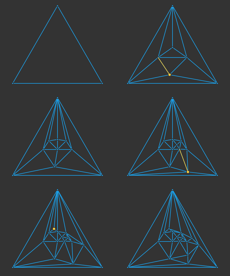
Here is the same sequence, with some details skipped and more points added:

More iterations of the Delaunay triangulation algorithm

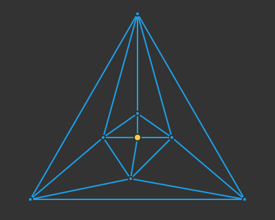
This algorithm starts with a bounding triangle that is large enough to contain all future points. The triangle is standalone, and so by definition is Delaunay:

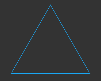
We start with a bounding triangle

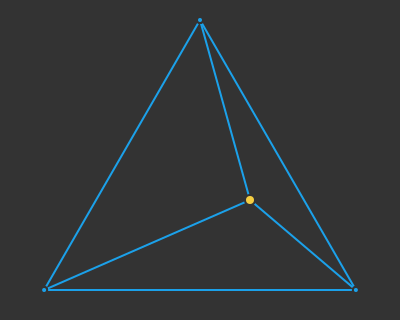
Every iteration of the Guibas & Stolfi algorithm inserts a new point into our mesh. We identify the triangle that new point is inside, and connect edges to the new point:

When adding a new point, first join it to its enclosing triangle

Note that in the special case where our new vertex is on an existing edge (or sufficiently close to an existing edge) we remove that edge and introduce four edges instead:

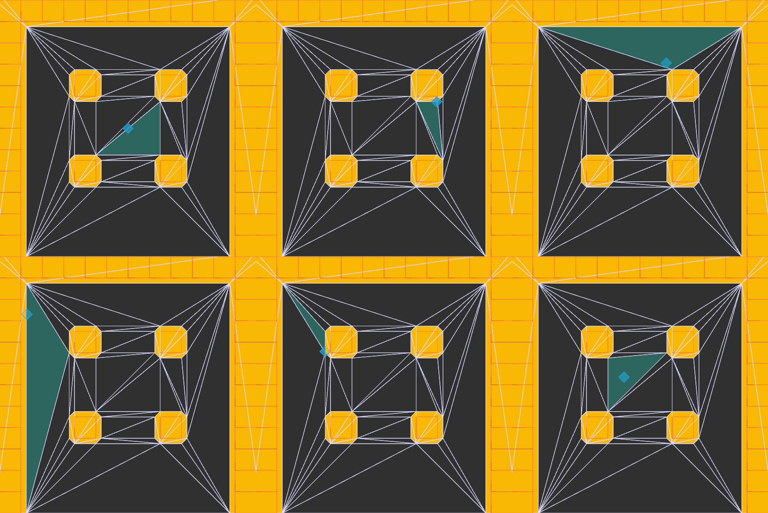
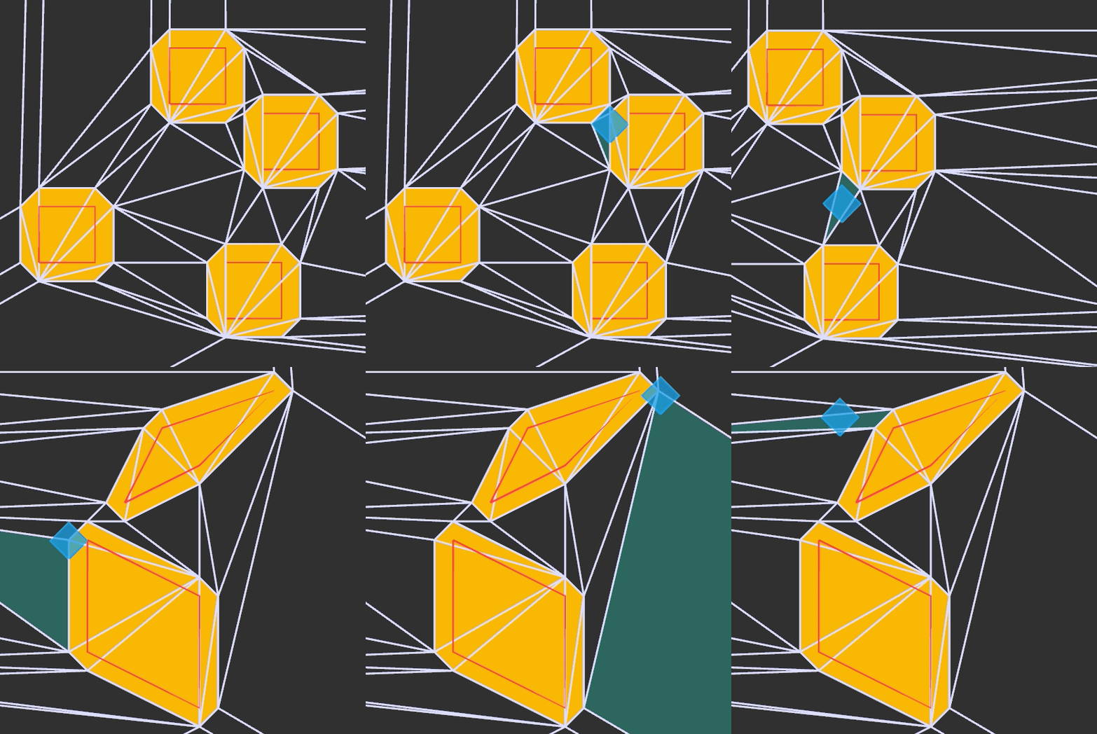
By introducing these new edges we have created three (or four) new triangles. These new triangles may no longer fulfill the Delaunay requirement of having vertices that are within some other triangle’s circumcircle.

Guibas & Stolfi noticed that the only possible violations occur between the new point and those opposite its surrounding face. That is, we need only walk around the edges of the triangle (or quadrilateral) that we inserted it into, and check whether we should flip those border edges in order to preserve the Delaunay condition.

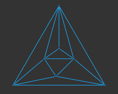
For example, for the new vertex above, we only need to check the four surrounding edges:

Here is an example where we need to flip an edge:

Interestingly, flipping an edge simply adds a new spoke to our new vertex. As such, we continue to only need to check the perimeter edges around the hub. This guarantees that we won’t propagate out and have to spend a lot of time checking edges, but instead just iterate around our one new point.

That’s one iteration of the algorithm. After that you just start the next iteration. Once you’re done adding points you remove the bounding triangle and you have your Delaunay triangulation.

The Data Structure

So the concept is pretty simple, but we all know that the devil is in the details. What really excited me about the Delaunay triangulation was the data structure used to construct it.

If we look at the algorithm, we can see what we might need our data structure to support:

  • Find the triangle enclosing a new point
  • Add new edges
  • Find vertices across from edges
  • Walk around the perimeter of a face

Okay, so we’ve got two concepts here – the ability to think about edges in our mesh, but also the ability to reason about faces in our mesh. A face, in this case, is usually a triangle, but it could also sometimes be a quadrilateral, or something larger.

The naive approach would be to represent our triangulation (i.e. mesh) as a a graph. That is, a list of vertices and a way to represent edge adjacency. Unfortunately, this causes problems. The edges would need to be ordered somehow to allow us to navigate the mesh.

The data structure of choice is called a quad-edge tree. It gives us the ability to quickly navigate both clockwise or counter-clockwise around vertices, or clockwise or counter-clockwise around faces. At the same time, quad-edge trees make it easy for new geometry to be stitched in or existing geometry to be removed.

Many of the drawings and explanations surrounding quad-edge trees are a bit complicated and hard to follow. I’ll do my best to make this explanation as tractable as possible.

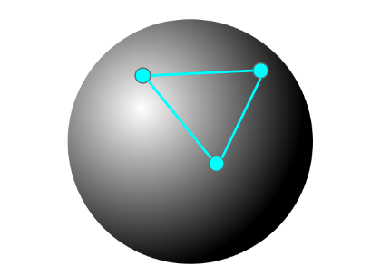
A quad-edge tree for 2D data represents a vertex mesh on a sphere:

A 2D mesh consisting of three vertices and three edges, on a 2D closed surface.

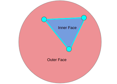
Said sphere is mostly irrelevant for what we are doing. In fact, we can think of it as very large. However, there is one important consequence of being on a sphere. Now, every edge between two vertices is between two faces. For example, the simple 2D mesh above has two faces:

Our 2D mesh has two faces – an outer face and an inner face. Each edge separates these two faces.

The quad-edge data structure can leverage this by associating each edge both with its two vertices and with its two faces, hence the name. Each real edge is represented as four directional edges in the quad-edge data structure: two directional edges between vertices and two directional edges between faces.

The quad-edge data structure represents each edge with four directional edges, two between vertices and two between faces.

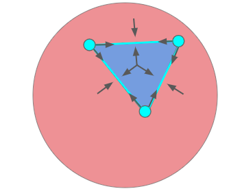
We can thus think of each face as being its own kind of special vertex:

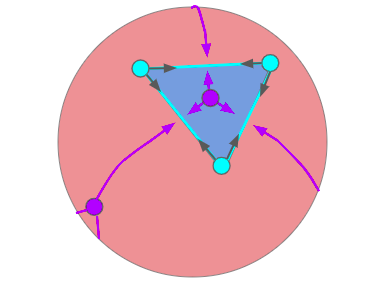
The purple vertices and arrows here are associated with the faces. We have one vertex for the inner face and one for the outer face.

As such, the quad-edge data structure actually contains two graphs – the directed graph of mesh edges and the dual graph that connects mesh faces. Plus, both of these graphs have inter-connectivity information in that each directed edge knows its left and right neighbors.

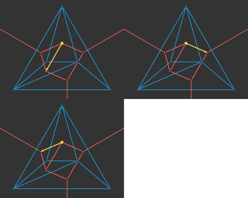
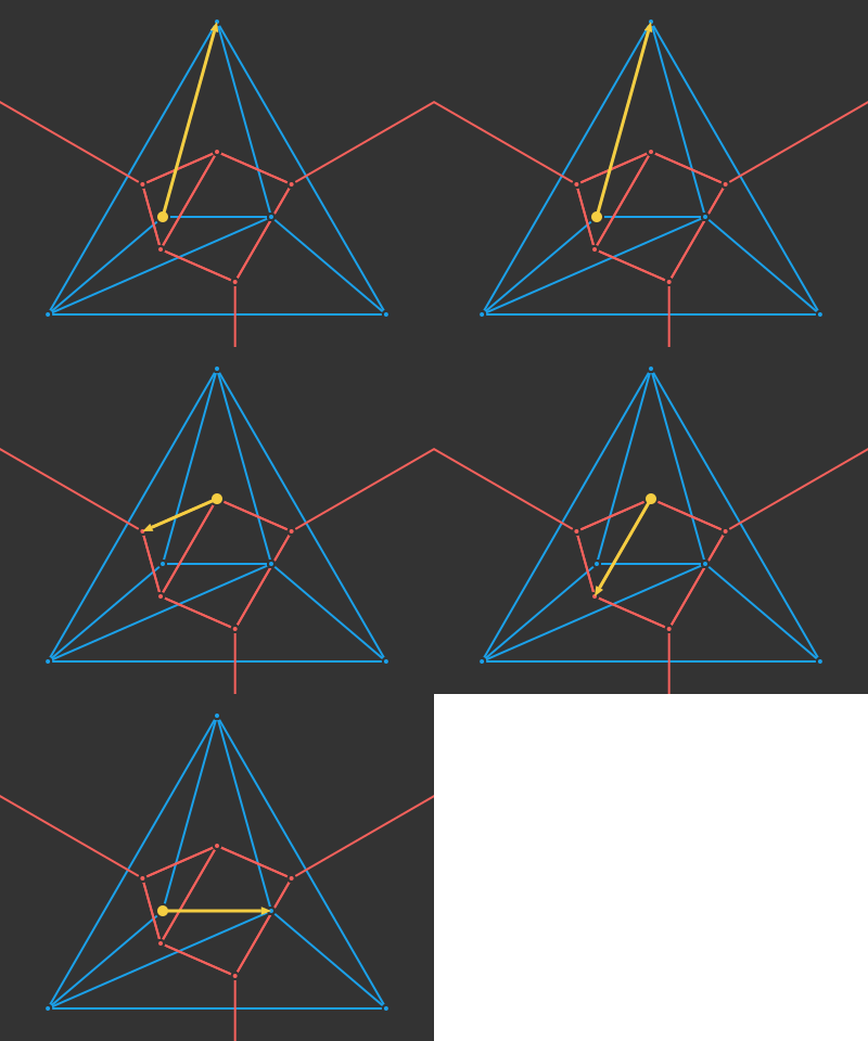
Okay, so pretty abstract. But, this gives us what we want. We can easily traverse the mesh by either flipping between the directed edges for a given mesh edge, or rotating around the base vertices for a given directed edge:

So now we are thinking about a special directed graph where each directed edge knows its left and right-hand neighbors and the other three directed edges that make up the edge in the original mesh:

struct QuarterEdge
    data::VertexIndex # null if a dual quarter-edge
    next_in_same_edge_on_right::QuarterEdgeIndex
    next_in_same_edge_on_left::QuarterEdgeIndex
    next_with_same_base_on_right::QuarterEdgeIndex
    next_with_same_base_on_left::QuarterEdgeIndex
end
struct Mesh
    vertices::Vector{Point}
    edges::Vector{QuarterEdge}
end

We have to update these rotational neighbors whenever we insert new edges into the mesh. It turns out we can save a lot of headache by dropping our left-handed neighbors:

struct QuarterEdge
    data::VertexIndex # null if a dual quarter-edge
    rot::QuarterEdgeIndex # next in same edge on right
    next::QuarterEdgeIndex # next with same base on right
end

We can get the quarter-edge one rotation to our left within the same edge simply by rotating right three times. Similarly, we can get the quater-edge one rotation to our left with the same base vertex by following rot – next – rot:

Rotating left around a vertex by following rot – next – rot.

Now we have our mesh data structure. When we add or remove edges, we have to be careful (1) to always construct new edges using four quarter edges whose rot entries point to one another, and (2) to update the necessary next entries both in the new edge and in the surrounding mesh. There are some mental hurdles here, but it isn’t too bad.

Finding the Enclosing Triangle

The first step of every Delaunay triangulation iteration involves finding the triangle enclosing the new vertex. We can identify a triangle using a quarter edge q whose base is associated with that face. If we do that, its three vertices, in counter-clockwise order, are:

  • A = q.rot.data
  • B = q.next.rot.data
  • C = q.next.next.rot.data

(Note that in code this looks a little different, because in Julia we would be indexing into the mesh arrays rather than following pointers like you would in C, but you get the idea).

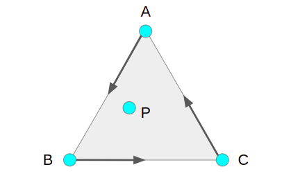
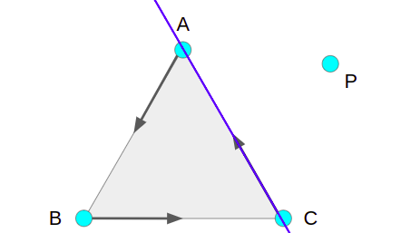
Suppose we start with some random face and extract its vertices A, B, and C. We can tell if our new point P is inside ABC by checking whether P is to the left of the ray AB, to the left of the ray BC, and to the left of the ray CA:

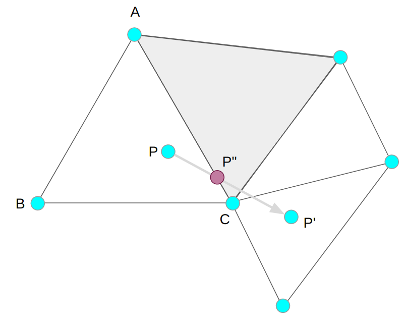
Checking whether P is left of a ray AB is the same as asking whether the triangle ABP has a counter-clockwise ordering. Conveniently, the winding of ABP is given by the determinant of a matrix:

\[\text{det}\left(\begin{bmatrix} A_x & A_y & 1 \\ B_x & B_y & 1 \\ P_x & P_y & 1 \end{bmatrix} \right)\]

If this value is positive, then we have right-handed (counter-clockwise) winding. If it is negative, then we have left-handed (clockwise) winding. If it is zero, then our points are colinear.

If our current face has positive windings then it encloses our point. If any winding is negative, the we know we can cross over that edge to get closer to our point.

Here triangle ABP and BCP have positive windings, but triangle CAP has a negative winding. As such, we need to cross the blue edge to get closer to P.

We simply iterate in this manner until we find our enclosing face. (I find this delightfully clean.)

Is a Point inside a Circumcircle

Checking whether vertices are inside circumcircles of triangles is central to the Delaunay triangulation process. The inspiring blog post has great coverage of why the following technique works, but if we want to check whether a point P is inside the circumcircle that passes through the (counter-clockwise-oriented) points of triangle ABC, then we need only compute:

\[\text{det}\left(\begin{bmatrix} A_x & A_y & A_x^2 + A_y^2 & 1 \\ B_x & B_y & B_x^2 + B_y^2 & 1 \\ C_x & C_y & C_x^2 + C_y^2 & 1 \\ P_x & P_y & P_x^2 + P_y^2 & 1 \end{bmatrix}\right)\]

If this value is positive, then P is inside the circumcircle. If it is negative, then P is external. If it is zero, then P is on its perimeter.

Some Last Implementation Details

I think that more or less captures the basic concepts of the Delaunay triangulation. There are a few more minor details to pay attention to.

First off, it is possible that our new point is exactly on an existing edge, rather than enclosed inside a triangle. When this happens, or when the new point is sufficiently close to an edge, it is often best to remove that edge and add four new edges. I illustrate this earlier in the post. That being said, make sure to never remove / split an original bounding edge. It is, after all, a bounding triangle.

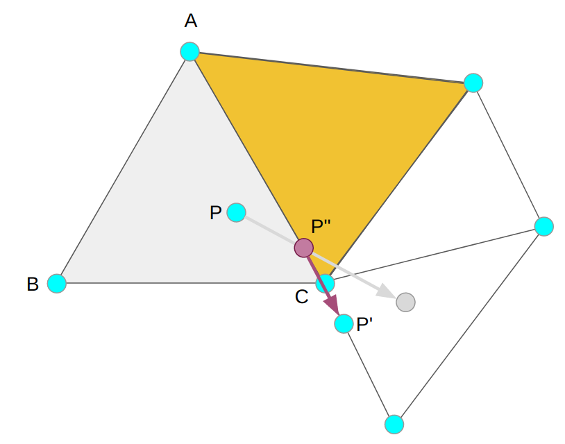
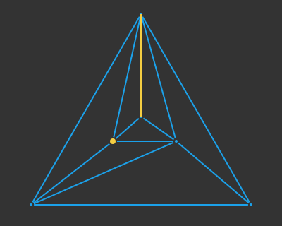
Second, after we introduce the new edges we have to consider flipping edges around the perimeter of the enclosing face. To do this, we simply rotate around until we arrive back where we started. The special cases here are bounding edges, which we never flip, and edges that connect to our bounding vertices, which we don’t flip if it would produce new triangles with clockwise windings:

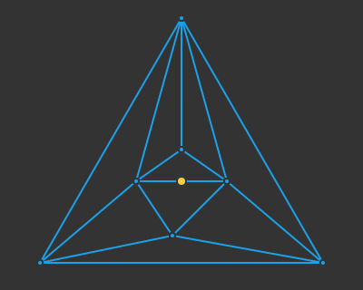
This newly added point (yellow) has an edge (also yellow) that cannot be flipped.

Once you’re done adding vertices, you remove the bounding triangle and any edges connected to it.

And all that is left as far as implementation details are concerned is the implementation itself! I put this together based on that other blog post as a quick side project, so it isn’t particularly polished. (Your mileage may vary). That being said, its well-visualized and I generally find reference implementations to be nice to have.

You can find the code here.

Conclusion

I thought the quad-edge data structure was really interesting, and I bet with some clever coding they could be really efficient as well. I really liked how solving this problem required geometry and visualization on top of typical math and logic skills.

Delaunay triangulations have a lot of neat applications. A future step might be to figure out constrained Delaunay triangulations for path-finding, or to leverage the dual graph to generate Voronoi diagrams.

How We Wrote Another Textbook

Hard copies of Algorithms for Decision Making (available in PDF form here for free) are shipping on August 16th! This book, the second one I have been fortunate to help write, was a large undertaking that spanned 4.5 years.

Back when Algorithms for Optimization came out, I wrote a blog post that detailed aspects of the special nature of our development setup. This blog post, 4 years later, is a look at how those aspects have changed for the second book.

But first, what is Algorithms for Decision Making, and how is it different than Algorithms for Optimization?

What Alg4DM is About

From the book website. I made the nifty cover art based on a POMDP solver evaluation tree.

Algorithms for Optimization covers the sort of decision making theory that one thinks of when considering modern artificial intelligence. Think Go AIs, aircraft collision avoidance, and using drones for wildfire suppression.

The book’s central focus is on the Markov Decision Process, or MDP. The MDP framework and its variants are simply general ways to frame decision making problems. For a problem to be represented as an MDP, you have to specify the problem’s states, its actions, how actions take you to successor states, and what rewards (or costs) you incur when doing so. Simple. The game 2048 can be formulated as an MDP, but so too can the problem of balancing investment portfolios.

Without going into too much detail (there’s an entire book, after all), the core insight of the MDP framework is that problems can be solved with dynamic programming according to the Bellman equation. All sorts of techniques stem from this, from optimal solvers for small discrete problems to fancy reinforcement learning techniques for large deep neural network policies.

The book has the following progression:

  • Starts with the basics of probability and utility, and introduces Bayesian networks and how to train them. (This is because BNs were used by Mykel for ACAS-X, and are a great way to represent transition models).
  • MDPs, including all sorts of fancy things including policy gradient optimization and actor-critic methods.
  • Model uncertainty, where we do not know the transition and reward functions ahead of time. There is some great content on imitation learning here too.
  • POMDPs, which extend MDPs to domains where we don’t observe the full state.
  • Multiagent systems, which involve problems with multiple decision-making agents. Think a bunch of robots jointly solving a problem together.

How Alg4DM is Different

Alg4DM took about 4.5 years between first commits to hard-copy. There were 3,417 commits to our git repository along with 826 filed issues. The printed book is 700 pages, with 225 color figures. In comparison, Alg4Opt is 500 pages, which makes the new book 40% longer.

While sheer size is a significant factor, there were other contributing complexities that made this book more challenging to write. I am proud to say that we still define the entire book in a LaTeX document and do all of figure generation and typesetting ourselves. We continued to use the Tufte LaTeX template. We typeset the book ourselves with LaTeX (as opposed to the publisher doing the typesetting), control our own lexing and styles, and have a suite of tests. We just had to overcome some additional hurdles to do so.

Interconnected Concepts (and Code)

Alg4DM crucially differs in how interconnected the material is. The chapters build on one another, with code from later chapters using or expanding on code from earlier chapters. These dependencies vastly increased the complexity of the work. We had to find unified representations that worked across the entire book, and any changes in one place could propagate to many others.

For example, the rollout method has an MDP version that accepts states and a POMDP method that accepts beliefs. Many POMDP methods call the state version, and thus depend on previous chapters.

Textbook-wide Codebase

When writing Alg4Opt, every chapter can be compiled alone, with standalone code. This made development pretty easy. We didn’t have any central shared code and could simply rely on pythontex blocks to execute Julia code for us:

A jlcode block that executes Julia code and produces a plot in the first book.

For Alg4DM, we needed later chapters to use the code from earlier chapters. As such, we needed a new tactic.

The approach we settled on was to construct a Julia package that would contain all of our code. This package would include both utility methods like plotting functions and example problem formulations, but also all of the code presented in the textbook. Algorithm blocks like the one below would be automatically detected and their contents exported into our package:

Blocks like the one above existed in Alg4Opt and resulted in typeset code, but that code never actually ran. We usually had extra copies of every algorithm that were used to _actually_ run and produce our figures. By scraping the book for our code, we could ensure that the code that was typeset was the code that we were actually using to generate our figures and run our tests. Furthermore, we could still compile chapters individually, as each chapter could just load the Julia package.

The end result looked basically like this:

Furthermore, we improved our test setup by writing tests directly inside the .tex files alongside everything else. These test blocks would also be parsed out during extraction, and could then be used to test our code:

Pretty simple, and it solved a lot of problems.

Now, it wasn’t without its trade-offs. First, whenever I was working on the book, I would have to remember to first run the extraction script to make sure that I had the latest and greatest. This added overhead, and forgetting to do it caused me some hours of pain.

Second, our base support code was stored in a different repository than the LaTeX for the book. This meant that another author could update the base code and I would have to remember to check out the latest Julia package to get those updates. Again, a pain point. Now that I know how to have Julia packages that aren’t stored in the standard Julia location, we can actually move our Julia package into the main book repo and avoid this issue.

Third, loading one large central package significantly increased book, and individual chapter, compile time. For Alg4Opt, each chapter only included the packages and code it needed. For Alg4DM, every chapter includes the entire support package, which has some hefty dependencies (such as Flux.jl). While we could do more work to split out the biggest dependencies, this fundamental increase in size would definitely still be noticeable. (Yes, package precompilation helps, but only so much).

Overall, I think our solution ended up being sufficient, but there are some improvements we could make moving forward.

Bigger, Fancier Problems

Many of the example problems and implementations behind the figures in Alg4Opt were relatively simple. They were mostly all 2D optimization problems, which are very quick to run. We could compile the book quickly and regenerate the figures every time without much hassle.

In Alg4DM that was no longer the case. Training an agent policy to solve a POMDP problem takes time, even for something as simple as the mountain-car problem. Compiling the book from scratch, including recompilation of all figures from the original Julia code, would take a very, very long time. As such, there are multiple cases where we had to save the .tex code produced for a particular figure, comment out the code that generated it, and include that instead:

An example of how a figure is loaded from its intermediary .tex file rather than being regenerated from source code every time.

This change was pretty seamless and easy to execute. It did not disrupt our workflow much. Furthermore, because we were still producing the PDF from .tex input, the figure would still be recompiled with the latest colors and formatting. The primary incurred overhead was remembering when to regenerate a figure because something underneath changed, such as the algorithm, something it calls, or the problem definition it was run on.

Breaking it Down in ways it hasn’t been Broken Down Before

The content covered in the optimization book was more intuitive for me, in many ways. While there certainly was some synthesis / repackaging of ideas, the amount of ground that had to be covered with respect to the new book was far greater.

The decision making book covers a large span of academic literature. We’ve got Bayesian networks, deep learning, traditional MDPs and POMDPs, imitation learning, reinforcement learning, multiagent planning, Markov games, and more. We needed consistent nomenclature that didn’t have overlapping concepts, while staying as true as possible to the literature. (For example, we spent a long time deciding what the symbol for a conditional plan would be. That issue took over a year to resolve.)

Furthermore, as with the first book, the 2nd book tries to cover the principle components of the algorithmic ideas. That is, we break down the little nuggets of progress. An algorithm like SARSOP has a lot of ideas inside of it, and we break those apart rather than presenting the SARSOP algorithm as a whole. Similarly, 1D optimization is often solved with Brent’s method, but you won’t find Brent’s method in our first book. You will, however, find the bisection, secant, and inverse quadratic interpolation methods – all methods that are used inside of Brent’s method.

Perhaps the greatest contribution this text makes is how we cover policy gradient optimization. We tease many of the concepts apart and present them individually in a way I haven’t seen before. The restricted gradient update naturally evolves into the natural gradient update, which evolves into a trust region update, etc. That chapter, and the actor-critic chapter thereafter, where the hardest ones for me to write, but I am quite happy with the result.

Conclusion

And that’s it! The new book is something I worked very hard on and it came out great. Mykel and Kyle worked very hard on it to, we got a ton of feedback from all sorts of helpful individuals, and we had great support from MIT Press and their editors.

I’ve been really fortunate to have been able to write this book with Mykel and Kyle. Decision-making is Mykel’s specialty, and Kyle has a lot of valuable multiagent knowledge (and is extremely detail-oriented and perceptive). I learned a lot doing the course of Alg4DM’s development, and I hope that its readers can learn a lot as well.
Packing Order Search for Sokoban

I spent a good while translating portions of the YASS Pascal code into Julia. I wanted to see how a larger, more sophisticated Sokoban solver works.

YASS (Yet Another Sokoban Solver), by Brian Damgaard, touts the use of a packing order calculation. I spent many hours trying to figure out what this was, and in the end boiled down the fundamental idea: it is a macro search where, instead of using individual box moves, the actions consist of either pushing a box all the way to a goal tile, or pushing a box as far away from its current position as possible with the hope that that frees up space for other boxes. That’s it.

Sokoban solvers typically reason about individual pushes. Above we show the legal pushes for the current game state.
The macro actions available from the start state. These actions allow us to push a box to a goal (as shown with the right box) or to two possible farthest-away tiles.

The devil, of course, is in the details. YASS has a lot of additional bells and whistles, such as using deadlock sets and a special phase in which a box comes from a relatively small area of the board. This post merely looks at the core idea.

A Coarser Problem Representation

As mentioned above, most Sokoban solvers reason about pushes. This is already a coarser problem representation than basic Sokoban, where the actions are individual player moves. The coarser representation significantly reduces the size of the search tree. The player can move in four directions, so by collapsing ten moves that lead to a box push we can nicely remove O(4^10) possible states in our search tree.

Generally speaking, reasoning with a coarser problem representation lets us tackle larger problems. The larger, “chunkier” actions let us get more done with less consideration. The trade-off is that we give up fine-tune adjustments. When it comes to player moves vs. box pushes this is often well worth it. For the macro moves in packing order calculations, that is less true. (More on that later).
A notional image showing search with a high-fidelity representation (blue, ex: player moves) versus search with a coarse representation (magenta, ex: push moves).
If we solve a problem in a coarser representation, we need to be able to transform it back into the finer representation:

We need to be able to transform from macro actions back to our finer representation.

Transforming box pushes back into player moves is easy, as we simply find the shortest path for the player to the appropriate side of the box, and then tack on the additional step to push the box. In this case, we have a well-defined way to find the (locally) optimal sequence of player moves in order to complete the push.

The macro actions taken in the pure version of the packing order calculation I implemented work the same way. We simply calculate the push distance between tiles and find the shortest push path to the destination tile. As such, packing order macro actions are converted to pushes, which in turn can be converted to player moves.

Packing Order Search

Search problems are defined by their states, actions, and goals. Our coarser problem for packing order search is:

States – the same as Sokoban, augmented with an additional state for each box. For each box, we keep track of whether it is:

  • unmoved
  • temporarily parked
  • permanently parked

Actions:

  • An unmoved box can either be temporarily parked or pushed all the way to a goal, assuming the destination is reachable only by pushing that box.
  • A temporarily parked box can be pushed all the way to a goal, assuming the destination is reachable only by pushing that box. (It cannot be temporarily re-parked.)

YASS computes up to two candidate temporary parking tiles for each box:

  • the farthest tile in Manhattan distance from the box’s current position
  • the farthest tile in push distance from the box’s current position

Goals – the same as Sokoban. All boxes on goals.

Several things are immediately apparent. First, we can bound the size of our search tree. Every box can be moved at most twice. As such, if we have b boxes, then we can have at most 2^b macro actions. This in turn makes it obvious that not every problem can be solved with this search method. The search method, as is, is incomplete. Many Sokoban problems require moving a single box multiple times before bringing it to a goal. We could counteract that by allowing multiple re-parks, but we quickly grow our search tree if we do so.

The number of actions in a particular state is fairly large. A single box can be pushed to every goal it can reach, and can be parked on up to two possible candidate tiles. Since the number of goals is the same as the number of boxes, this means we have up to (2+b)^b actions in a single state. (Typically far less than that). As such, our tree is potentially quite fanned out. (In comparison, solving for box pushes has at most 4b actions in a single state).

Here we see how the two lower-right boxes each only have one stashing location, but the upper-left box can be pushed to any goal or stashed next to the goals. (Note that we do not stash boxes in tiles from which they cannot be retrieved.)

We can apply pretty much any of the basic search algorithms from my previous post to this coarser problem representation. I just went with a basic depth-first search.

Below we can see a solution for a basic 3-box problem, along with its backed-out higher-fidelity versions:

While illustrative and a neat experience, this basic depth-first packing order search is not particularly great at solving Sokoban problems. It does, however, nicely illustrate the idea of translating between problem representations.

Reverse Packing Order Search

The packing order calculation done by YASS performs its search in reverse. That is, rather than starting with the initial board state and trying to push boxes to goals, it starts with all boxes on goals and tries to pull them to their starting states.

Reverse search and its various forms (ex: bidirectional search), are motivated by the fact that searching in the forward direction alone may not be as easy as the reverse direction. One common example is a continuous-space path finding problem in which the search has to find a way through a directional bottleneck:

A search from the start to the goal would likely have trouble to finding its way through the narrow opening, whereas a search from the goal to the start can be nicely funneled out.

The motivation for a reverse search in Sokoban is similar. However, rather than having to thread the needle through directional bottlenecks, Sokoban search has to avoid deadlock states. Reverse search is motivated by the idea that it is easier to get yourself into a deadlock state by pushing boxes than it is to get yourself into deadlock states by pulling boxes. This technique is presented in this paper by Frank Takes. Note that deadlocks are still possible – they just occur less frequently. That being said, 2×2 deadlocks won’t occur, the box cannot be pulled up against a wall or in a corner, etc.

The starting state in a reverse search is a goal state – all boxes on goals. Note that we do not know where the player should start – they would end up next to one of the boxes. As such, we have to consider all player-reachable regions surrounding the goals. Below we show the initial state for a problem and three possible reverse search start states:

My simple solver simply tries each possible start state until it finds a solution (or fails after exhausting all possibilities).

Reverse packing order search does perform better than packing order search. It still suffers from incompleteness, and would need to be fleshed out with more bells and whistles to be useful (deadlock analysis, goal room packing, etc.). That being said, we can solve some problems that are too big for my previous version of A*, such as Sasquatch 49. We solve it in 0.002s.

Macro Actions (Pulls)
The push solution backed out from the macro-pull solution.
The player-move solution.

So there you have it, a simple solver that can handle an 8-box problem. Granted, it cannot solve most 8-box problems, but we have blazed a bit of a trail forward.

Conclusion

Code is available here.

The main takeaway here is that one of the best ways to scale to larger problems is to reason with a coarser problem representation. We don’t plan every footstep when deciding to walk to the kitchen. Similarly, we reason about overall street routes when planning to drive somewhere, rather than thinking about every lane change (usually). Multi-level planning can be incredibly powerful – we just have to be careful to be able to back out feasible solutions, and not miss important details.

Propulsive Landing

Let’s work through how one might (in a broad sense) write a controller for guiding rockets under propulsive control for a pinpoint landing. Such a “planetary soft landing” is central to landing exploratory rovers and some modern rockets. It is also quite an interesting optimization problem, one that starts off seemingly hairy but turns out to be completely doable. There is something incredible about landing rockets, and there is something awesome and inspiring about the way this math problem lets us do just that.

Everything in this post is based off of Lars Blackmore’s paper, Lossless Convexification of Nonconvex Control Bound and Pointing Constraints of the Soft Landing Optimal Control Problem.

Problem Setup

We have a rocket. Our rocket is falling fast, and we wish to have it stop nice and gently on the surface of our planet. We will get it to stop gently by having the rocket use its thruster (or thrusters) to both slow itself down and navigate to a desired landing location.

As such, our problem is to find a thrust control profile \(\boldsymbol{T}_c\) to produce a trajectory from an initial position \(\boldsymbol{r}_0\) and initial velocity \(\dot{\boldsymbol{r}}_0\) to a final position at the landing pad with zero final velocity. As multiple trajectories may be feasible, we’ll choose the one that minimizes our fuel use.

We model the rocket as a point-mass. This is done both because it is a lot easier, but also because rockets are pretty stable and we want to maintain a vertical orientation, and any attitude control that we would need has much faster-acting dynamics that we could control separately.

Dynamics

Our state at a given point in time is given by both the physical state \(\boldsymbol{x} = [\boldsymbol{r}, \dot{\boldsymbol{r}}]\) consisting of the position and the velocity, and the rocket’s mass \(m\). I am going to do the derivation in 2D, but it is trivial to extend all of this to the 3D case.

Our physical system dynamics are:

\[\dot{\boldsymbol{x}}(t) = \boldsymbol{A} \boldsymbol{x}(t) + \boldsymbol{B} \left(\boldsymbol{g} + \frac{\boldsymbol{T}_c(t)}{m(t)}\right)\]

where \(\boldsymbol{g}\) is the gravity vector and our matrices are:

\[\boldsymbol{A} = \begin{bmatrix} \boldsymbol{0} & \boldsymbol{I} \\ \boldsymbol{0} & \boldsymbol{0} \end{bmatrix} \qquad \boldsymbol{B} = \begin{bmatrix} \boldsymbol{0} & \boldsymbol{0} \\ \boldsymbol{I} & \boldsymbol{0} \end{bmatrix}\]

for input vectors \([\boldsymbol{r}, \dot{\boldsymbol{r}}]\).

Our mass dynamics are \(\dot{m} = -\alpha \|\boldsymbol{T}_c(t)\|\), where the mass simply decreases in proportion to the thrust. Here \(\alpha\) is the constant thrust-specific fuel consumption that determines our rate of mass loss per unit of thrust.

Let us assume that we specify the time until landing, such that \(t\) runs from zero to \(t_f\).

Adding Constraints

We can take these dynamics and construct an optimization problem that finds a thrust control profile that brings us from our initial state to our final state with the minimum amount of fuel use. There are, however, a few additional constraints that we need to add.

First, we do not want our rocket to go below ground. The way this was handled in the paper was by adding a simple glide-slope constraint that prevents the rocket’s position from ever leaving a cone above the landing location. This ensure that we remain a safe distance above the ground. In 2D this is:

\[r_y(t) \geq \tan(\gamma_\text{gs}) r_x(t) \quad \text{for all } t\]

where \(r_x(t)\) and \(r_y(t)\) are our horizontal and vertical positions at time \(t\), and \(\gamma_\text{gs} \in [0,\pi/2]\) is a glide slope angle.

Next, we need to ensure that we do not use more fuel than what we have available. Let \(m_\text{wet}\) be our wet mass (initial rocket mass, consisting of the rocket plus all fuel), and \(m_\text{dry}\) be our dry mass (just the mass of the rocket – no fuel). Then we need our mass to remain above \(m_\text{dry}\).

Finally, we have some constraints with respect to our feasible thrust. First off, we cannot produce more thrust than our engine provides: \(\|\boldsymbol{T}_c\| \leq \rho_2\). Secondarily, we also cannot produce less thrust than a certain minimum: \(0 < \rho_1 \leq \|\boldsymbol{T}_c\|\). This lowerbound is caused by many rocket engines being physically unable to reduce thrust to zero without going out. Unfortunately, it is a non-convex constraint, and we will have to work around it later.

The thrust magnitude constraints are nonconvex, because we can draw a line between two feasible points and get a non-feasible point.

The last thrust constraint has to do with how far we can actuate our rocket engines. We are keeping our rocket vertically aligned during landing, and often have a limited ability to gimbal the engine. We introduce a thrust-pointing constraint that limits our deviation from vertical to within an angle \(\theta\):

\[ \boldsymbol{T}_{c,y}(t) \geq \|\boldsymbol{T}_c(t)\| \cos(\theta) \]

Our basic nonconvex minimum fuel landing problem is thus:

\[\begin{matrix}\text{minimize}_{\boldsymbol{T}_c} & \int_0^{t_f} \alpha \|\boldsymbol{T}_c(t)\| \> dt & & \\ \text{subject to} & \dot{\boldsymbol{x}}(t) = \boldsymbol{A} \boldsymbol{x}(t) + \boldsymbol{B} \left(\boldsymbol{g} + \frac{\boldsymbol{T}_c(t)}{m(t)}\right) & \text{for all } t \in [0, t_f] & \text{physical dynamics} \\ & \dot{m} = -\alpha \|\boldsymbol{T}_c(t)\| & \text{for all } t \in [0, t_f] & \text{mass dynamics} \\ & 0 < \rho_1 \leq \|\boldsymbol{T}_c\| \leq \rho_2 & \text{for all } t \in [0, t_f] & \text{thrust magnitude bounds} \\ & \boldsymbol{T}_{c,y}(t) \geq \|\boldsymbol{T}_c(t)\| \cos(\theta) & \text{for all } t \in [0, t_f] & \text{thrust pointing constraint} \\ & r_y(t) \geq \tan(\gamma_\text{gs}) r_x(t)& \text{for all } t \in [0, t_f] & \text{glide slope constraint} \\ & \boldsymbol{r}(0) = \boldsymbol{r}_0, \dot{\boldsymbol{r}}(0) = \dot{\boldsymbol{r}}_0 & & \text{physical initial conditions} \\ & m(0) = m_\text{wet} & & \text{mass initial condition} \\ & \boldsymbol{r}(t_f) = [0,0], \dot{\boldsymbol{r}}(t_f) = [0,0] & & \text{physical final conditions} \\ & m(t_f) \geq m_\text{dry} & & \text{mass final condition} \end{matrix}\]

Lossless Convexification

The basic problem formulation above is difficult to solve because it is nonconvex. Finding a way to make it convex would make it far easier to solve.

Our issues are the nonconvex thrust bounds and the division by mass in our dynamics.

To get around the thrust bounds, we introduce an additional slack variable, \(\Gamma(t)\). We use this slack variable in our thrust bounds constraint and mass dynamics, and constrain our actual thrust magnitude to lie below \(\Gamma\):

\[\dot{m}(t) = -\alpha \Gamma\]

\[\|\boldsymbol{T}\|_c(t) \leq \Gamma(t)\]

\[0 < \rho_1 \leq \Gamma(t) \leq \rho_2\]

\[ \boldsymbol{T}_{c,y}(t) \geq \cos(\theta) \Gamma(t) \]

Introducing the slack variable has formed a convex feasible region. Note that, suddenly, thrusts that were previously illegal are now legal (those with small magnitude). However, the problem definition guarantees that our optimal solution will lie on the surface of this truncated cone. All such points satisfy the thrust bounds. I think this is one of the coolest parts of the whole derivation.

On the one hand, we have introduced a new time-varying quantity, and have thus increased the complexity of our problem. However, by introducing this quantity, we have made our constraints convex. This trade-off will be well worth it.

We can get around the nonconvex division by mass with a change of variables:

\[\sigma \equiv \frac{\Gamma}{m} \qquad \boldsymbol{u} \equiv \frac{\boldsymbol{T}_c}{m} \qquad z \equiv \ln m\]

This simplifies our dynamics to:

\[\dot{\boldsymbol{x}}(t) = \boldsymbol{A} \boldsymbol{x}(t) + \boldsymbol{B} \left(\boldsymbol{g} + \boldsymbol{u}(t)\right)\]

\[ \dot{z}(t) = -\alpha \sigma(t) \]

Unfortunately, our thrust bounds constraint becomes nonconvex:

\[0 \leq \rho_1 e^{-z(t)} \leq \sigma(t) \leq \rho_2 e^{-z(t)}\]

We can convexify it by approximating the constraint with a 2nd-order Taylor expansion of \(e^{-z(t)}\):

\[\rho_1 e^{-z_o(t)} \left(1 – (z(t) – z_o(t)) + \frac{1}{2}(z(t) – z_o(t))^2\right) \leq \sigma(t) \leq \rho_2 e^{-z_o(t)} \left(1 – (z(t) – z_o(t)) \right)\]

where \(z_o(t) = \ln (m_\text{wet} – \alpha \rho_2 t)\).

The left-hand side forms a second-order cone constraint, which have the form \(\|x\|_2 \leq t\). Quadratic constraints can be converted to such second-order cone constraints.

We thus end up with the following convex problem:

\[\begin{matrix}\text{minimize}_{\boldsymbol{u}, \boldsymbol{\sigma}} & \int_0^{t_f} \sigma(t) \> dt & & \\ \text{subject to} & \dot{\boldsymbol{x}}(t) = \boldsymbol{A} \boldsymbol{x}(t) + \boldsymbol{B} \left(\boldsymbol{g} + \boldsymbol{u}(t)\right) & \text{for all } t \in [0, t_f] & \text{physical dynamics} \\ & \dot{z} = -\alpha \sigma(t) & \text{for all } t \in [0, t_f] & \text{mass dynamics} \\ & \|\boldsymbol{u}(t)\| \leq \sigma(t) & \text{for all } t \in [0, t_f] & \text{slack variable bound} \\ & \rho_1 e^{-z_o(t)} \left(1 – (z(t) – z_o(t)) + \frac{1}{2}(z(t) – z_o(t))^2\right) \leq \sigma(t) & \text{for all } t \in [0, t_f] & \text{thrust magnitude, lower} \\ & \sigma(t) \leq \rho_2 e^{-z_o(t)} \left(1 – (z(t) – z_o(t)) \right) & \text{for all } t \in [0, t_f] & \text{thrust magnitude, upper} \\ & u_y(t) \geq \sigma(t) \cos(\theta) & \text{for all } t \in [0, t_f] & \text{thrust pointing constraint} \\ & r_y(t) \geq \tan(\gamma_\text{gs}) r_x(t)& \text{for all } t \in [0, t_f] & \text{glide slope constraint} \\ & \boldsymbol{r}(0) = \boldsymbol{r}_0, \dot{\boldsymbol{r}}(0) = \dot{\boldsymbol{r}}_0 & & \text{physical initial conditions} \\ & z(0) = \ln m_\text{wet} & & \text{mass initial condition} \\ & \boldsymbol{r}(t_f) = [0,0], \dot{\boldsymbol{r}}(t_f) = [0,0] & & \text{physical final conditions} \\ & z(t_f) \geq \ln m_\text{dry} & & \text{mass final condition} \end{matrix}\]

It can be shown that if there is a feasible solution to the first problem, then that solution also defines a feasible solution to this new problem. Furthermore, this solution is an optimal solution of the new problem. (This is related to the fact that \(\boldsymbol{u}\) is not minimized – we only care about minimizing \(\boldsymbol{\sigma}\), but for physical feasibility we end up needing \(\boldsymbol{u} = \boldsymbol{\sigma}\)).

Discretization in Time

The final problem transformation involves moving from a continuous formulation to a discrete formulation, such that we can actually implement a numerical algorithm. We discretize time into \(n\) equal-width periods such that \(n \Delta t = t_f\):

\[t^{(k)} = k \Delta t, \qquad k = 0, \ldots, n\]

Our thrust profile is a continuous function of time. We construct it as a combination of \(n+1\) basis functions, \(\phi_{0:n}\):

\[\begin{bmatrix}\boldsymbol{u}(t) \\ \sigma(t)\end{bmatrix} = \sum_{k=0}^n \boldsymbol{p}^{(k)} \phi^{(k)}(t), \qquad t \in [0,t_f]\]

where the \(\boldsymbol{p}^{(k)} \in \mathbb{R}^3\) are mixing weights that we will optimize. Note that we did not have to have as many basis functions as discrete points – it just makes the math easier. Various basis functions can be used, but the paper uses the sawtooth:

\[\phi_j(t) = \begin{cases} \frac{t_j-t}{\Delta t} & \text{for } t \in [t_{j-1}, t_j] \\ \frac{t – t_j}{\Delta t} & \text{for } t \in [t_{j}, t_{j+1}] \\ 0 & \text{otherwise} \end{cases}\]

Our system state is \([\boldsymbol{r}(t)^\top, \dot{\boldsymbol{r}}(t)^\top, z(t)]^\top\) with the continuous-time system dynamics:

\[\begin{split} \begin{bmatrix} \dot{\boldsymbol{r}}(t) \\ \ddot{\boldsymbol{r}}(t) \\ \dot{z}(t) \end{bmatrix} & = \begin{bmatrix} \boldsymbol{0} & \boldsymbol{I} & 0 \\ \boldsymbol{0} & \boldsymbol{0} & 0 \\ 0 & 0 & 0 \end{bmatrix} \begin{bmatrix} \boldsymbol{r}(t) \\ \dot{\boldsymbol{r}}(t) \\ z(t) \end{bmatrix} + \begin{bmatrix} \boldsymbol{0} & \boldsymbol{0} \\ \boldsymbol{I} & \boldsymbol{0} \\ 0 & -\alpha \end{bmatrix} \begin{bmatrix} \boldsymbol{u}(t) \\ \sigma(t) \end{bmatrix} + \begin{bmatrix} \boldsymbol{0} \\ \boldsymbol{g} \\ 0 \end{bmatrix} \\ \dot{\mathtt{x}(t)} & = \boldsymbol{A}_c \mathtt{x}(t) + \boldsymbol{B}_c \mathtt{u}(t) + \mathtt{g} \end{split} \]

In order to discretize, we would like to have a linear equation to get our state at every discrete time point. We know that the solution to the ODE \(\dot{x} = a x + b u\) is:

\[ x(t) = e^{at} x_0 + \int_0^t e^{A(t-\tau)} b u(\tau) \> d\tau \]

Similarly, the solution to our ODE is:

\[ \mathtt{x}(t) = e^{\boldsymbol{A_c}t} \mathtt{x}_0 + \int_0^t e^{\boldsymbol{A_c}(t-\tau)} \left(\boldsymbol{B}_c \mathtt{u}(\tau) + \mathtt{g}\right) \> d\tau \]

We can get our discrete update by plugging in \(\Delta t\):

\[ \mathtt{x}(\Delta t) = e^{\boldsymbol{A_c}\Delta t} \mathtt{x}_0 + \int_0^{\Delta t} e^{\boldsymbol{A_c}(\Delta t-\tau)} \left(\boldsymbol{B}_c \mathtt{u}(\tau) + \mathtt{g}\right) \> d\tau \]

If we’re going from \(k\) to \(k+1\), we get:

\[ \mathtt{x}^{(k+1)} = e^{\boldsymbol{A_c}\Delta t} \mathtt{x}^{(k)} + \int_0^{\Delta t} e^{\boldsymbol{A_c}(\Delta t-\tau)} \left(\boldsymbol{B}_c \mathtt{u}(\tau) + \mathtt{g}\right) \> d\tau \]

We then substitute in our basis function formulation:

\[ \begin{split} \mathtt{x}^{(k+1)} &= \left[e^{\boldsymbol{A_c}\Delta t}\right] \mathtt{x}^{(k)} + \int_0^{\Delta t} e^{\boldsymbol{A_c}(\Delta t-\tau)} \left(\boldsymbol{B}_c \left( \boldsymbol{p}^{(k)} \phi^{(k)}(t) + \boldsymbol{p}^{(k+1)} \phi^{(k+1)}(t) \right) + \mathtt{g}\right) \> d\tau \\ & = \left[e^{\boldsymbol{A_c}\Delta t}\right] \mathtt{x}^{(k)} + \int_0^{\Delta t} e^{\boldsymbol{A_c}(\Delta t-\tau)} \left(\boldsymbol{B}_c \left( \left( 1- \frac{\tau}{\Delta t}\right) \boldsymbol{p}^{(k)} + \left( \frac{\tau}{\Delta t}\right) \boldsymbol{p}^{(k+1)} \right) + \mathtt{g}\right) \> d\tau \\ & = \left[e^{\boldsymbol{A_c}\Delta t}\right] \mathtt{x}^{(k)} + \left[\int_0^{\Delta t} e^{\boldsymbol{A_c}(\Delta t-\tau)} \boldsymbol{B}_c\right] \left( \boldsymbol{p}^{(k)} + \mathtt{g} \right) + \left[\int_0^{\Delta t} e^{\boldsymbol{A_c}(\Delta t-\tau)} \boldsymbol{B}_c \frac{\tau}{\Delta t}\right] \left( \boldsymbol{p}^{(k+1)} – \boldsymbol{p}^{(k)} \right) \\ &= \boldsymbol{A}_d \texttt{x}^{(k)} + \boldsymbol{B}_{d1} \left( \boldsymbol{p}^{(k)} + \mathtt{g} \right) + \boldsymbol{B}_{d2} \left( \boldsymbol{p}^{(k+1)} – \boldsymbol{p}^{(k)} \right) \end{split} \] Our discrete update equation is thus also linear. We can compute our matrices once using numerical methods for integration. We can apply our relation recursively to get our state at any discrete time point. All of these updates are linear:

\[\begin{split} \mathtt{x}^{(1)} & = \boldsymbol{A}_d \texttt{x}^{(0)} + \boldsymbol{B}_{d1} \left( \boldsymbol{p}^{(0)} + \mathtt{g} \right) + \boldsymbol{B}_{d2} \left( \boldsymbol{p}^{(1)} – \boldsymbol{p}^{(0)} \right) \\ \mathtt{x}^{(2)} & = \boldsymbol{A}_d \texttt{x}^{(1)} + \boldsymbol{B}_{d1} \left( \boldsymbol{p}^{(1)} + \mathtt{g} \right) + \boldsymbol{B}_{d2} \left( \boldsymbol{p}^{(2)} – \boldsymbol{p}^{(1)} \right) \\ &= \boldsymbol{A}_d \left(\boldsymbol{A}_d \texttt{x}^{(0)} + \boldsymbol{B}_{d1} \left( \boldsymbol{p}^{(0)} + \mathtt{g} \right) + \boldsymbol{B}_{d2} \left( \boldsymbol{p}^{(1)} – \boldsymbol{p}^{(0)} \right)\right) + \boldsymbol{B}_{d1} \left( \boldsymbol{p}^{(1)} + \mathtt{g} \right) + \boldsymbol{B}_{d2} \left( \boldsymbol{p}^{(2)} – \boldsymbol{p}^{(1)} \right) \\ &= \boldsymbol{A}_d^2 \texttt{x}^{(0)} + \left(\boldsymbol{B}_{d1} + \boldsymbol{A}_d \boldsymbol{B}_{d1}\right) \mathtt{g} + \left(\boldsymbol{A}_d \boldsymbol{B}_{d1} – \boldsymbol{A}_d \boldsymbol{B}_{d2} \right) \boldsymbol{p}^{(0)} + \left(\boldsymbol{B}_{d1} + \boldsymbol{A}_d \boldsymbol{B}_{d2} – \boldsymbol{B}_{d2} \right) \boldsymbol{p}^{(1)} + \boldsymbol{B}_{d2} \boldsymbol{p}^{(2)} \\ & \enspace \vdots \end{split}\]

Note that due to our choice of basis function, \(\boldsymbol{u}^{(k)} = [p_1^{(k)} p_2^{(k)}]^\top\) and \(\sigma^{(k)} = p_3^{(k)}\).

We can approximate the continuous version of our objective function:

\[ \int_0^{t_f} \sigma(t) \> dt \approx \sum_{k=0}^n p^{(k)}_3\]

We can pull all of this together and construct a discrete-time optimization problem. We optimize the vector \(\boldsymbol{\eta}\), which simply contains all of the \(\boldsymbol{p}\) vectors:

\[\boldsymbol{\eta} = \begin{bmatrix} \boldsymbol{p}^{(0)} \\ \boldsymbol{p}^{(1)} \\ \vdots \\ \boldsymbol{p}^{(n)} \end{bmatrix} \]

Our problem is:

\[\begin{matrix}\text{minimize}_{\boldsymbol{\eta}} & \sum_{k=0}^n p^{(k)}_3 & & \\ \text{subject to} & \mathtt{x}^{(k+1)} = \boldsymbol{A}_d \texttt{x}^{(k)} + \boldsymbol{B}_{d1} \left( \boldsymbol{p}^{(k)} + \mathtt{g} \right) + \boldsymbol{B}_{d2} \left( \boldsymbol{p}^{(k+1)} – \boldsymbol{p}^{(k)} \right) & \text{for all } k \in [0, 1, \ldots, n-1] & \text{dynamics} \\ & \|[p_1^{(k)} p_2^{(k)}]^\top\| \leq p_3^{(k)} & \text{for all } k \in [0, 1, \ldots, n] & \text{slack variable bound} \\ & \rho_1 e^{-z_o(k \Delta t)} \left(1 – (z(k \Delta t) – z_o(k \Delta t)) + \frac{1}{2}(z(k \Delta t) – z_o(k \Delta t))^2\right) \leq \sigma(k \Delta t) & \text{for all } k \in [0, 1, \ldots, n] & \text{thrust magnitude, lower} \\ & \sigma(k \Delta t) \leq \rho_2 e^{-z_o(k \Delta t)} \left(1 – (z(k \Delta t) – z_o(k \Delta t)) \right) & \text{for all } k \in [0, 1, \ldots, n] & \text{thrust magnitude, upper} \\ & p_2^{(k)} \geq p_3^{(k)} \cos(\theta) & \text{for all } k \in [0, 1, \ldots, n] & \text{thrust pointing constraint} \\ & r_y(k \Delta t) \geq \tan(\gamma_\text{gs}) r_x(k \Delta t)& \text{for all } k \in [0, 1, \ldots, n-1] & \text{glide slope constraint} \\ & \boldsymbol{r}(0) = \boldsymbol{r}_0, \dot{\boldsymbol{r}}(0) = \dot{\boldsymbol{r}}_0 & & \text{physical initial conditions} \\ & z(0) = \ln m_\text{wet} & & \text{mass initial condition} \\ & \boldsymbol{r}(t_f) = [0,0], \dot{\boldsymbol{r}}(t_f) = [0,0] & & \text{physical final conditions} \\ & z(t_f) \geq \ln m_\text{dry} & & \text{mass final condition} \end{matrix}\]

This final formulation is a finite-dimensional second-order cone program (SOCP). It can be solved by standard convex solvers to get a globally-optimal solution.

Note that we only apply our constraints at the discrete time points. This tends to be sufficient, due to the linear nature of our dynamics.

Coding it Up

I coded this problem up using cvxpy. My python notebook is available here.


Update: I originally did the implementation in Julia, but found odd behavior with the Convex.jl solvers I was using. I tried both SCS (the default recommended solver for Convex.jl) and COSMO. Neither of these solvers worked for the propulsive landing problem. Both solvers had the same behavior – they would find a solution that satisfied the terminal conditions, but would fail to satisfy the other constraints. Giving it more iterations would cause it to slowly make progress on the other constraints, but eventually it would give up and decide the problem is infeasible.

Prof. Kochenderfer noticed that Julia didn’t work for me, and recommended that I try ECOS. I swapped that in and it just worked. My Julia notebook is available here.


import cvxpy as cp
import numpy as np
import scipy

We define our parameters, which I adapted from the paper:

m_wet = 2000.0        # rocket wet mass [kg]
m_dry =  300.0        # rocket dry mass [kg]
thrust_max = 24000.0  # maximum thrust
ρ1 = 0.2 * thrust_max # lower bound on thrust
ρ2 = 0.8 * thrust_max # upper bound on thrust
α = 5e-4              # rocket specific impulse [s]
θ = np.deg2rad(30)    # max thrust angle deviation from vertical [rad]
γ = np.deg2rad(15)    # no-fly bounds angle [rad]
g = 3.71              # (martian) gravity [m/s2]
tf = 52.0             # duration of the simulation [s]
n_pts = 50            # number of discretization points
 
# initial state (x,y,x_dot,y_dot,z)
x0 = np.array([600.0, 1200.0, 50.0, -95.0, np.log(m_wet)])

We then compute some derived parameters:

t = np.linspace(0.0, tf, n_pts) # time vector [s]
N = len(t) - 2                  # number of control nodes
dt = t[1] - t[0]

We compute \(\boldsymbol{A}_c\) and \(\boldsymbol{A}_d\):

Ac = np.vstack((
        np.hstack((np.zeros((2, 2)), np.eye(2),        np.zeros((2, 1)))),
        np.hstack((np.zeros((2, 2)), np.zeros((2, 2)), np.zeros((2, 1)))),
        np.zeros((1, 5))
     ))
 
Ad = scipy.linalg.expm(Ac * dt)

We compute \(\boldsymbol{B}_c\), \(\boldsymbol{B}_{d1}\), and \(\boldsymbol{B}_{d2}\):

def integrate_trapezoidal(f, a, b, n):
    retval = f(a) * 0.5 + f(b) * 0.5
    for k in range(1, n):
        retval = retval + f(a + k*(b-a)/n)
    retval = retval * (b - a)/ n
    return retval
 
Bc = np.vstack((
        np.hstack((np.zeros((2, 2)), np.zeros((2, 1)))),
        np.hstack((np.eye(2),        np.zeros((2, 1)))),
        np.hstack((np.zeros((1, 2)), np.reshape(np.array([]), (1, 1))))
    ))
 
Bd1 = integrate_trapezoidal(lambda s: np.matmul(scipy.linalg.expm(Ac*(dt-s)), Bc), 0.0, dt, 10000)
Bd2 = integrate_trapezoidal(lambda s: np.matmul(scipy.linalg.expm(Ac*(dt-s))*(s/dt), Bc), 0.0, dt, 10000)

We implement our recursive calculation for the state at time index \(k\):

# gravitational 3-vector [m/s2]
g3 = np.array([0.0, -g, 0.0])
 
def get_xk(Ad, Bd1, Bd2, η, x0, g3, k):
    xk = x0
    p_km1 = np.array([0.0,0.0,0.0])
    p_k = η[0:3]
    ind_low = 0
    for j in range(0,k):
        xk = np.matmul(Ad,xk) + np.matmul(Bd1, (p_km1 + g3)) + np.matmul(Bd2, (p_k - p_km1))
        p_km1 = p_k
        ind_low = min(ind_low+3, 3*(N+1))
        p_k = η[ind_low : ind_low+3]
    return xk

and we define our problem:

# Create the CVX problem 
η = cp.Variable(3*N)
 
ω = np.tile(np.array([0,0,1]), N) # only minimize the σ's
 
# minimize fuel consumption
objective = cp.Minimize(ω.T@η)
constraints = []
 
# thrust magnitude constraints
for k in range(0, N):
    j = 3*k
    constraints.append(cp.norm(η[j:j+2]) <= η[j+2])
 
# thrust cant angle constraints
for k in range(0, N):
    j = 3*k
    uy = η[j+1]
    σ = η[j+2]
    constraints.append(uy >= np.cos(θ) * σ)
 
# thrust slack variable lower and upper bounds
z0 = lambda k: np.log(m_wet - α*ρ2*dt*k)
for k in range(0, N):
    j = 3*k
    σk = η[j+2]
    xk = get_xk(Ad, Bd1, Bd2, η, x0, g3, k)
    zk = xk[-1]
 
    a = ρ1 * np.exp(-z0(k))
    z0k = z0(k).item()
    z1k = z1(k).item()
 
    constraints.append(a * (1 - (zk-z0k) + 0.5*cp.square(zk-z0k)) <= σk)    
    constraints.append(σk <= ρ2 * np.exp(-z0k) * (1 - (zk-z0k)))
 
# glide angle constraints
for k in range(1, N):
    j = 3*k
    xk = get_xk(Ad, Bd1, Bd2, η, x0, g3, k)
    constraints.append(xk[1] >= np.tan(γ) * xk[0])
 
# terminal conditions
xf = get_xk(Ad, Bd1, Bd2, η, x0, g3, N)
constraints.append(xf[0:4] == [0,0,0,0])
constraints.append(xf[4] >= np.log(m_dry))
 
prob = cp.Problem(objective, constraints)

and we solve it!

result = prob.solve()
print(prob.status)

We can extract our solution (thrust profile and trajectory) as follows:

η_eval = η.value
 
xk = np.zeros((len(x0), len(t)))
for (i,k) in enumerate(range(0,N)):
    xk[:,i] = get_xk(Ad, Bd1, Bd2, η_eval, x0, g3, k)
 
xs = xk[0,:]
ys = xk[1,:]
us = xk[2,:]
vs = xk[3,:]
zs = xk[4,:]
 
mass = np.exp(zs)
 
u1 = η_eval[0::3]
u2 = η_eval[1::3]
σ = η_eval[2::3]
 
Tx = u1 * mass
Ty = u2 * mass
Γ = σ * mass
thrust_mag = [np.hypot(Tyi, Txi) for (Txi, Tyi) in zip(Tx, Ty)]
thrust_ang = [np.arctan2(Txi, Tyi) for (Txi, Tyi) in zip(Tx, Ty)]

The plots end up looking pretty great. Here is the landing trajectory we get for the code above:

The blue line shows the rocket’s position over time, the orange line shows the no-fly boundary, and the black line shows the ground (\(y = 0\)). The rocket has to slow down so as to avoid the no-fly zone (orange), and then nicely swoops in for the final touchdown. Here is the thrust profile:

Our thrust magnitude matches our slack variable \(\Gamma\), as expected for optimal trajectories. We also see how the solution “rides the rails”, hitting both the upper and lower bounds. This is very common for optimal control problems – we use all of the control authority available to us.

The two thrust components look like this:

We see that \(T_y\) stays positive, as it should. However, \(T_x\) starts off negative to move the rocket left, and then counters in order to stick the landing.

Our thrust angle stays within bounds:

We can of course play around with our parameters and initial conditions to get different trajectories. Here is what happens if we flip the initial horizontal velocity:

Here is what happens if we increase the minimum thrust to \(\rho_1 = 0.3 T_\text{max}\):

How to Avoid Specifying the Trajectory Duration

One remaining issue with the convex formulation above is that we have to specify our trajectory duration, \(t_f\). This, and \(n\), determine \(\Delta t\) and our terminal condition, both of which are pretty central to the problem.

We might be interested, for example, in finding the minimum-time landing trajectory. Typically, the longer the trajectory, the more fuel that is used, so being able to reduce \(t_f\) automatically can have big benefits.

The naive approach is to do a search over \(t_f\) in order to find the smallest valid trajectory duration. In fact, this is exactly what the authors suggest:

Once we have a procedure to compute the fuel optimal trajectory for a given time-of-flight, \(t_f\), we use the Golden search algorithm to determine the time-of-flight with the least fuel need, \(t^*_f\). This line search algorithm is motivated by the observation that the minimum fuel is a unimodal function of time with a global minimum

Behcet Acikmese, Lars Blackmore, Daniel P. Scharf, and Aron Wolf

I would be surprised if there were a way to optimize for \(t_f\) alongside the trajectory, but there very well could be a better approach!

The Curious Case of the Missing Constraint

As a final note, I wanted to mention that there are some additional constraints in some versions of the paper. Notably, this paper includes these constraints in its “Problem 3”:

\[ \log\left(m_\text{wet} – \alpha \rho_2 t\right) \leq z(t) \leq \log\left(m_\text{wet} – \alpha \rho_1 t\right) \]

These constraints do not appear in Lossless Convexification of Nonconvex Control Bound and Pointing Constraints of the Soft Landing Optimal Control Problem.

After thinking about it, I don’t think the constraints are needed. They are enforcing that our mass lies between an upper and lower bound. The upperbound is the mass we would have if we had minimum thrust for the entire trajectory, whereas the lowerbound is the mass we would have if we had maximum thrust for the entire trajectory. The fact that we constrain our thrusts (and constrain our final mass) mean that we don’t really need these constraints.

Conclusion

I find this problem fascinating. We go through a lot of math, so much that it can be overwhelming, but it all works out in the end. Every step ends up being understandable and justifiable. I then love seeing the final trajectories play out, and get the immediate feedback in the trajectory as we adjust the initial conditions and constraints.

I hope you enjoyed this little side project.

Push-Permutation Optimization of Sokoban Solutions

My last few blog posts covered methods for getting push-optimal solutions to simple Sokoban puzzles. Traditional Sokoban, however, operates on player moves. Solvers often reason about pushes to simplify decision-making. Unfortunately, push-optimal solutions are not necessarily move-optimal. For example, this solution is push-optimal but has some very clear inefficiencies when we render out the player moves required to travel between boxes:

Push-Optimal (but not move-optimal) solution for a subset of Sokoban 01
Rendering the same push-optimal solution above with its player moves clearly shows how inefficient it is

Directly solving for move-optimal solutions from scratch is difficult. Rather than doing that, it is common to optimize a given solution to try to find another solution with a smaller player move count. Thus, Sokoban solvers typically find push-optimal solutions, or more commonly some valid solution, and Sokoban optimizers work with an existing solution to try and improve it.

There are many approaches for optimizing solutions. In this post, I’ll just cover some very basic approaches to improve my push-optimal solutions from the previous posts.

Solution Evaluation

Every optimization problem needs an objective function. Here, we are trying to find solutions with fewer player moves. As such, our objective function takes in a potential push sequence solution and evaluates both its validity (whether it is, in fact, a solution), and the number of player moves. The number of player moves is the number of box pushes plus the number of moves to walk to the appropriate location for each push.

All of the strategies I use here simply shuffle the pushes around. I do not change the pushes. As we’ll see, this basic assumption works pretty well for the problems at hand.

We thus have a simple constrained optimization problem – to minimize the number of player moves by permuting the pushes in a provided push-optimal solution subject to the constraint that we maintain solution integrity. We can easily evaluate a given push sequence for validity by playing the game through with that push sequence, which we have to do anyway to calculate the number of player moves.

Strategy 1: Consider all Neighboring Box Pairs

The simplest optimization strategy is to try permuting neighboring push pairs. We consider neighboring pairs because they are temporally close, and thus more likely to be a valid switch. Two pushes that are spread out a lot in time are likely to not be switchable – other pushes are more likely to have to happen in-between.

This strategy is extremely simple. Just iterate over all pushes, and if two neighboring pushes are for two different boxes, try swapping the push order and then evaluating the new push sequence to see if it solves the problem with a smaller move count. If it does, keep the new solution.

For example, if our push sequence, in terms of box pushes, is AAABBCCBAD, we would evaluate AABABCCBAD first, and it does not lead to an improvement, consider AAABCBCBAD next, etc.

Strategy 2: Consider all Neighboring Same-Box Sequences

The strategy above is decent for fine-tuning the final solution. However, by itself it is often unable to make big improvements.

Move-optimal solutions are often achieved by grouping pushes for the same box together. This intuitively leads to the player not having to trek to other boxes between pushes – they are already right next to the box they need to push next. We thus can do quite well by considering moving chunks of pushes for the same box around rather than moving around a single box push at a time.

This approach scans through our pushes, and every time we change which box we are pushing, considers moving forward all push sequences of all other next boxes to before the current sequence of box pushes. For example, if our push sequence is AAABBCCBAD, we would consider BBAAACCBAD, CCAAABBBAD, and DAAABBCCBA, greedily keeping the first one that improves our objective.

Strategy 3: Group Same-Box Push Sequences

The third basic strategy that I implemented moves box sub-sequences in addition to full box sequences in an effort to consolidate same-box push sequences. For each push, if the next push is not for the same box, we find the next push sequence for this box and try to move the largest possible sub-sequence for that box to immediately after our current push – i.e., chaining pushes.

For example, if our push sequence is AAABBCCBAD, we would consider AAAABBCCBD, and if that did not lead to an improvement, would consider AAABBBCCAD.

Similarly, if our push sequence is AAABBAAA, we would consider AAAAAABB, then AAAAABBA, and finally AAAABBAA in an effort to find the largest sub-sequence we could consolidate.

Putting it All Together

None of these heuristics are particularly sophisticated or fancy. However, together we get some nice improvements. We can see the improvement on the full Sokoban 01 problem:

Full Push-Optimal Solution for Sokoban 01: 97 box pushes and 636 player moves
After re-ordering the pushes we have 260 only player moves

The following output shows how the algorithm progressed:

iteration, push count, number of applications of strategy 1, ... strategy 2, ... strategy 3:
1: 636  0  0  0
dbcffffffffccfffcddccadfcccddbcbaaccdccadddbaddadedaaddaaaebaaaabbddaaeeeeebbeeeebbeeebbbbbbbeebb
2: 598  4  0  1
dbcfffffffffffcccddccadfcccddcbbaacdcccadddbadadeddaaddaaaebaaaabbddaaeeeeebbeeeebbeeebbbbbbbeebb
3: 520  7  0  2
dbcffffffffffffcccddccadcccddcbbaadccccadddbdaaedddaaddaaaebaaaabbddaaeeeeebbeeeebbeeebbbbbbbeebb
4: 504  8  0  3
dbcffffffffffffcccccddadcccddcbbaadccccaddbddaaedddaaddaaaebaaaabbddaaeeeeebbeeeebbeeebbbbbbbeebb
5: 482  8  0  4
dbcffffffffffffccccccccddadddcbbaadccccaddbddaaedddaaddaaaebaaaabbddaaeeeeebbeeeebbeeebbbbbbbeebb
6: 470  8  0  5
dbcffffffffffffcccccccccddadddbbaadccccaddbddaaedddaaddaaaebaaaabbddaaeeeeebbeeeebbeeebbbbbbbeebb
7: 450  8  0  6
dbcffffffffffffcccccccccccccddadddbbaadaddbddaaedddaaddaaaebaaaabbddaaeeeeebbeeeebbeeebbbbbbbeebb
8: 428  9  0  7
dbcffffffffffffcccccccccccccdddddabbaaadddbddaaedddaaddaaaebaaaabbddaaeeeeebbeeeebbeeebbbbbbbeebb
9: 428  9  0  8
dbcffffffffffffcccccccccccccdddddaabbaadddbddaaedddaaddaaaebaaaabbddaaeeeeebbeeeebbeeebbbbbbbeebb
10: 420  9  0  9
dbcffffffffffffcccccccccccccdddddaabbaadddddbaaedddaaddaaaebaaaabbddaaeeeeebbeeeebbeeebbbbbbbeebb
11: 404  9  0  10
dbcffffffffffffcccccccccccccdddddaabbaaddddddddbaaeaaddaaaebaaaabbddaaeeeeebbeeeebbeeebbbbbbbeebb
12: 376  9  0  11
dbcffffffffffffcccccccccccccdddddaabbaaddddddddddbaaeaaaaaebaaaabbddaaeeeeebbeeeebbeeebbbbbbbeebb
13: 376  9  0  12
dbcffffffffffffcccccccccccccdddddaabbaaddddddddddddbaaeaaaaaebaaaabbaaeeeeebbeeeebbeeebbbbbbbeebb
14: 358  9  0  13
dbcffffffffffffcccccccccccccdddddaabbaaddddddddddddbaaaaaaaeebaaaabbaaeeeeebbeeeebbeeebbbbbbbeebb
15: 344  9  0  14
dbcffffffffffffcccccccccccccdddddaabbaaddddddddddddbaaaaaaaaaaaeebbbaaeeeeebbeeeebbeeebbbbbbbeebb
16: 320  9  0  15
dbcffffffffffffcccccccccccccdddddaabbaaddddddddddddbaaaaaaaaaaaaaeebbbeeeeebbeeeebbeeebbbbbbbeebb
17: 302  9  0  16
dbcffffffffffffcccccccccccccdddddaabbaaddddddddddddbaaaaaaaaaaaaaeeeeeeebbbbbeeeebbeeebbbbbbbeebb
18: 286  9  0  17
dbcffffffffffffcccccccccccccdddddaabbaaddddddddddddbaaaaaaaaaaaaaeeeeeeeeeeebbbbbbbeeebbbbbbbeebb
19: 260  9  0  18
dbcffffffffffffcccccccccccccdddddaabbaaddddddddddddbaaaaaaaaaaaaaeeeeeeeeeeeeeebbbbbbbbbbbbbbeebb
20: 260  9  0  19
dbcffffffffffffcccccccccccccdddddaabbaaddddddddddddbaaaaaaaaaaaaaeeeeeeeeeeeeeeeebbbbbbbbbbbbbbbb

So there you have a quick-and-dirty way to get some nicer solutions out of our push-optimal solutions. Other approaches will of course be needed once we have solutions that aren’t push-optimal, which we’ll get once we move onto problems that are too difficult to solve optimally. There we’ll have to do more than just permute the pushes around, but actually try changing our push sequence and refining our solution more generally.

For those interested, the Sokoban Optimizer “Scribbles” by Brian Damgaard are an excellent resource.

Sokoban Reach and Code Performance

In my previous post, I covered some basic Sokoban search algorithms and some learnings from my digging into YASS (Yet Another Sokoban Solver). I covered the problem representation but glossed over how we determine the pushes available to us in a given board state. In this post, I cover how we calculate that and then conduct into a bunch of little efficiency investigations.

A push-optimal solution to a Sokoban puzzle

Set of Actions

We are trying to find push-optimal solutions to Sokoban problems. That is, we are trying to get every box on a box in the fewest number of pushes possible. As such, the actions available to us each round are the set of pushes that our player can conduct from their present position:

The set of pushes the player (red star) can conduct from their present position

Our Sokoban solver will need to calculate the set of available pushes in every state. As such, we end up calculating the pushes a lot, and the more efficient we are at it, the faster we can conduct our search.

A push is valid if:

  • our player can reach a tile adjacent to the block from their current position
  • the tile opposite the player, on the other side of the block, is free

As such, player reachability is crucial to the push calculation.

Reachablity for the same game state as the previous image. Red tiles are player-reachable, and green tiles are reachable boxes.

Above we see the tiles reachable from the player’s position (red) and the boxes adjacent to player-reachable tiles. This view is effectively the output of our reachability calculation.

Efficient Reach Calculations

The set of reachable tiles can be found with a simple flood-fill starting from the player’s starting location. We don’t care about the shortest distance, just reachability, so this can be achieved with either a breadth-first or a depth-first traversal:

Naive Reach Calculation

Let’s look at a naive Julia implementation using depth-first traversal:

function calc_reachable_tiles(game::Game, board::Board, □_start::TileIndex)
   min_reachable_tile = □_start
   reachable_tiles = Set{TileIndex}()
   reachable_boxes = Set{TileIndex}()
   to_visit = TileIndex[]
 
   push!(reachable_tiles, □_start)
   push!(to_visit, □_start)
 
   while !isempty(to_visit)
      # pop stack
      □ = pop!(to_visit)
 
      # Examine tile neighbors
      for dir in DIRECTIONS
         ▩ = □ + game.step_fore[dir]
         if ((board[] & WALL) == 0) && (▩ ∉ reachable_tiles)
            if ((board[] & BOX) == 0)
                push!(to_visit, ▩)
                push!(reachable_tiles, ▩)
                min_reachable_tile = min(min_reachable_tile, □_start)
            else
                push!(reachable_boxes, ▩)
            end
         end
      end
   end
 
   return (reachable_tiles, reachable_boxes, min_reachable_tile)
end

This code is somewhat inefficient, most notably in that it allocates sets for both reachable_tiles and reachable_boxes, which change in size during its execution. (We also compute the minimum reachable tile, for use in state hashing, as explained in the previous post.) Let’s evaluate its runtime on this large puzzle:

A large test puzzle based on Sasquatch 49. All tiles are initially reachable

Using @btime from BenchmarkTools.jl, we get 15.101 μs (28 allocations: 9.72 KiB). Honestly, 15 microseconds is actually quite good – much better than I expected from a naive implementation. That being said, let’s see if we can do better.

YASS Reach Calculation with Preallocated Memory

I spent a fair amount of time investigating YASS, which was written in Pascal. The Pascal code was structured differently than most of the code bases I’ve worked with. The working memory is declared and allocated at the top of the file in a global space, and is then used throughout. This preallocation makes it incredibly efficient. (As an aside, it was quite difficult to tell where variables were defined, since the naming conventions didn’t make it clear what was declared locally and what was global, and Pascal scoping really threw me into a loop). I feel that a lot of modern programming gets away with assuming we have a lot of memory, and is totally fine with paying the performance cost. However, in tight inner loops like this reach calculation, which might run many hundreds of thousands of times, we care enough about performance to pay special attention.

The Julia performance tips specifically call out paying attention to memory allocations. The previous code allocated 9.72 KiB. Let’s try to knock that down.

We’ll start by defining a struct that holds our preallocated memory. Rather than keeping lists or sets of player-reachable tiles and boxes, we’ll instead store a single flat array of tiles the same length as the board. This representation lets us just flag a given tile as a player-reachable tile or a player-reachable box:

mutable struct ReachableTiles
    # The minimum (top-left) reachable tile. Used as a normalized player position
    min_reachable_tile::TileIndex 
    # Incremented by 2 in each reach calculation
    # The player-reachable tiles have the value 'calc_counter'
    # Tiles with neighboring boxes have the value 'calc_counter' + 1
    # Non-floor tiles are set to typemax(UInt32)
    calc_counter::UInt32
    tiles::Vector{UInt32}
end

This data structure lets us store everything we care about, and does not require clearing between calls (only once we get to wraparound). We just increment a counter and overwrite our memory with every call.

is_reachable(□::Integer, reach::ReachableTiles) = reach.tiles[] == reach.calc_counter
is_reachable_box(□::Integer, reach::ReachableTiles) = reach.tiles[] == reach.calc_counter + 1

The reachability calculation from before can now be modified to update our ReachableTiles struct:

function calc_reachable_tiles!(
    reach::ReachableTiles,
    game::Game,
    board::Board,
    □_start::TileIndex,
    stack::Vector{TileIndex}
  )::Int
 
    # The calc counter wraps around when the upper bound is reached
    if reach.calc_counter ≥ typemax(UInt32) - 2
        clear!(reach, board)
    end
 
    reach.calc_counter += 2
    reach.min_reachable_tile = □_start
    reach.tiles[□_start] = reach.calc_counter
    n_reachable_tiles = 1
 
    # depth-first search uses a stack
    stack[1] = □_start
    stack_hi = 1 # index of most recently pushed item
 
    # stack contains items as long as stack_hi > 0
    while stack_hi > 0
        # pop stack
        □ = stack[stack_hi]
        stack_hi -= 1
 
        # Examine tile neighbors
        for dir in DIRECTIONS
            ▩ = □ + game.step_fore[dir]
            if reach.tiles[] < reach.calc_counter
                # An unvisited floor tile, possibly with a box
                # (non-floors are typemax ReachabilityCount)
                if (board[] & BOX) == 0 # not a box
                    n_reachable_tiles += 1
                    # push the square to the stack
                    stack_hi += 1
                    stack[stack_hi] = ▩
                    reach.tiles[] = reach.calc_counter
                    reach.min_reachable_tile = min(▩, reach.min_reachable_tile)
                else
                    # a box
                    reach.tiles[] = reach.calc_counter + 1
                end
            end
        end
    end
 
    reach.calculated = true
    return n_reachable_tiles
end

This time, @btime gives us 2.490 μs (2 allocations: 224 bytes), which is about 6x faster and a massive reduction in allocations.

I was particularly pleased by the use of the stack memory passed into this method. Our depth-first traversal has to keep track of tiles that need to be expanded. The code uses a simple vector to store the stack, with just a single index variable stack_hi that points to the most recently pushed tile. We know that we will never have more items in the stack than tiles on our board, so stack can simply be the same length as our board. When we push, we increment stack_hi and place our item there. When we pop, we grab our item from stack[stack_hi] and then decrement. I loved the elegance of this when I discovered it. Nothing magic or anything, just satisfyingly clean and simple.

Avoiding Base.iterate

After memory allocations, the other thing common culprit of inefficient Julia code is a variable with an uncertain / wavering type. At the end of the day, everything ends up as assembly code that has to crunch real bytes in the CPU, so any variable that can be multiple things necessarily has to be treated in multiple ways, resulting in less efficient code.

Julia provides a @code_warntype macro that lets one look at a method to see if anything has a changing type. I ran it on the implementation above and was surprised to see an internal variable with a union type, @_9::Union{Nothing, Tuple{UInt8, UInt8}}.

It turns out that for dir in DIRECTIONS is calling Base.iterate, which returns either a tuple of the first item and initial state or nothing if empty. I was naively thinking that because DIRECTIONS was just 0x00:0x03 that this would be handled more efficiently. Anyways, I was able to avoid this call by using a while loop:

dir = DIR_UP
while dir <= DIR_RIGHT
    ...
    dir += 0x01
end

That change drops us down to 1.989 μs (2 allocations: 224 bytes), which is now about 7.5x faster than the original code. Not bad!

Graph-Based Board Representation

Finally, I wanted to try out a different board representation. The code about stores the board, a 2d grid, as a flat array. To move left we decrement our index, to move right we increment our index, and to move up or down we change by our row length.

I looked into changing the board to only store the non-wall tiles and represent it as a graph. That is, have a flat list of floor tiles and for every tile and every direction, store the index of its neighbor in that direction, or zero otherwise:

struct BoardGraph
    # List of tile values, one for each node
    tiles::Tiles
 
    # Index of the tile neighbor for each tile.
    # A value of 0 means that edge is invalid.
    neighbors::Matrix{TileIndex} # tile index × direction
end

This form has the advantage of a smaller memory footprint. By dropping the wall tiles we can use about half the space. Traversal between tiles should be about as expensive as before.

The reach calculation looks more or less identical. As we’d expect, the performance is close to the same too: 2.314 μs (4 allocations: 256 bytes). There is some slight inefficiency, perhaps because memory lookup is not as predictable, but I don’t really know for sure. Evenly structured grid data is a nice thing!

Pushes

Once we’ve done our reachable tiles calculation, we need to use it to compute our pushes. The naive way is to just iterate over our boxes and append to a vector of pushes:

function get_pushes(game::Game, s::State, reach::ReachableTiles)
    pushes = Push[]
    for (box_number, □) in enumerate(s.boxes)
        if is_reachable_box(□, reach)
            # Get a move for each direction we can get at it from,
            # provided that the opposing side is clear.
            for dir in DIRECTIONS
                □_dest = □ + game.step_fore[dir] # Destination tile
                □_player = □ - game.step_fore[dir] # Side of the player
                # If we can reach the player's pos and the destination is clear.
                if is_reachable(□_player, reach) && ((s.board[□_dest] & (FLOOR+BOX)) == FLOOR)
                    push!(pushes, Push(box_number, dir))
                end
            end
        end
    end
    return pushes
end

We can of course modify this to use preallocated memory. In this case, we pass in a vector pushes. The most pushes we could have is four times the number of boxes. We allocate that much and have the method return the actual number of boxes:

function get_pushes!(pushes::Vector{Push}, game::Game, s::State, reach::ReachableTiles)::Int
    n_pushes = 0
    for (box_number, □) in enumerate(s.boxes)
        if is_reachable_box(□, reach)
            # Get a move for each direction we can get at it from,
            # provided that the opposing side is clear.
            for dir in DIRECTIONS
                □_dest = □ + game.step_fore[dir] # Destination tile
                □_player = □ - game.step_fore[dir] # Side of the player
                # If we can reach the player's pos and the destination is clear.
                if is_reachable(□_player, reach) && ((s.board[□_dest] & (FLOOR+BOX)) == FLOOR)
                    n_pushes += 1
                    pushes[n_pushes] = Push(box_number, dir)
                end
            end
        end
    end
    return n_pushes
end

Easy! This lets us write solver code that looks like this:

n_pushes = get_pushes!(pushes, game, s, reach)
for push_index in 1:n_pushes
    push = pushes[push_index]
    ...
end

An alternative is to do something similar to Base.iterate and generate the next push given the previous push:

"""
Given a push, produces the next valid push, with pushes ordered
by box_index and then by direction.
The first valid push can be obtained by passing in a box index of 1 and direction 0x00.
If there no valid next push, a push with box index 0 is returned.
"""
function get_next_push!(
    game::Game,
    s::State,
    reach::ReachableTiles,
    push::Push = Push(1, 0)
  )
    box_index = push.box_index
    dir = push.dir
    while box_index ≤ length(s.boxes)
        □ = s.boxes[box_index]
        if is_reachable_box(□, reach)
            # Get a move for each direction we can get at it from,
            # provided that the opposing side is clear.
            while dir < N_DIRS
                dir += one(Direction)
                □_dest = game.board_start.neighbors[□, dir]
                □_player = game.board_start.neighbors[□, OPPOSITE_DIRECTION[dir]]
                # If we can reach the player's pos and the destination is clear.
                if □_dest > 0 && 
                   □_player > 0 &&
                   is_reachable(□_player, reach) &&
                   not_set(s.tiles[□_dest], BOX)
                    return Push(box_index, dir)
                end
            end
        end
 
        # Reset
        dir = 0x00
        box_index += one(BoxIndex)
    end
 
    # No next push
    return Push(0, 0)
end

We can then use it as follows, without the need to preallocate a list of pushes:

push = get_next_push!(game, s, reach)
while push.box_index > 0
    ...
    push = get_next_push!(game, s, reach, push)
end

Both this code and the preallocated pushes approach are a little annoying, in a similar what that changing for dir in DIRECTIONS to a while loop is annoying. They uses up more lines than necessary and thus makes the code harder to read. That being said, these approaches are more efficient. Here are solve times using A* with all three methods on Sasquatch 02:

  • naive: 17.200 μs
  • Preallocated pushes: 16.480 μs
  • iterator: 15.049 μs

Conclusion

This post thoroughly covered how to compute the player-reachable tiles and player-reachable boxes for a given Sokoban board. Furthermore, we used this reachability to compute the valid pushes. We need the pushes in every state, so we end up computing both many times during a solver run.

I am surprised to say that my biggest takeaway is actually that premature optimization is the root of all evil. I had started this Sokoban project keen on figuring out how YASS could solve large Sokoban problems as effectively as possible. I spent a lot of time learning about its memory representations and using efficient preallocated memory implementations for the Julia solver.

I would never have guessed that the difference between a naive implementation and an optimized implementation for the reach calculation would merely yield a 7.5x improvement. Furthermore, I would never have thought that the naive implementation for getting the pushes would be basically the same as using a preallocated vector. There are improvements, yes, but it really goes to show that these improvements are really only worth it if you really measure your code and really need that speed boost. The sunk development time and the added code complexity is simply not worth it for a lot of everyday uses.

So far, the search algorithm used has had a far bigger impact on solver performance than memory allocation / code efficiencies. In some ways that makes me happy, as algorithms represent “how we go about something” and the memory allocation / efficiencies are more along the lines of implementation details.

As always, programmers need to use good judgement, and should look at objective data.