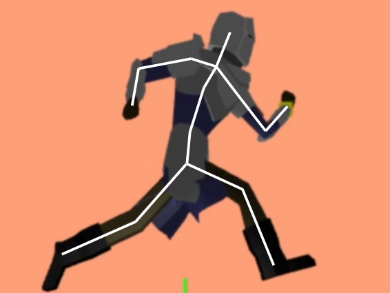
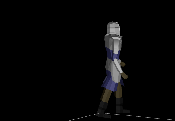
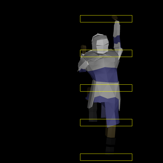
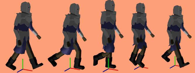
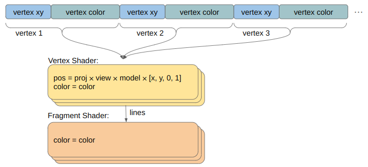
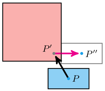
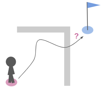
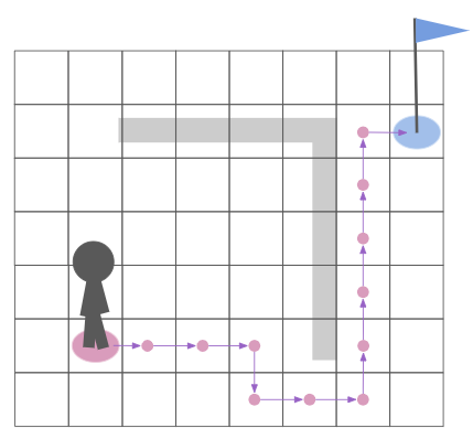
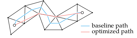
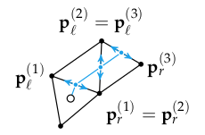
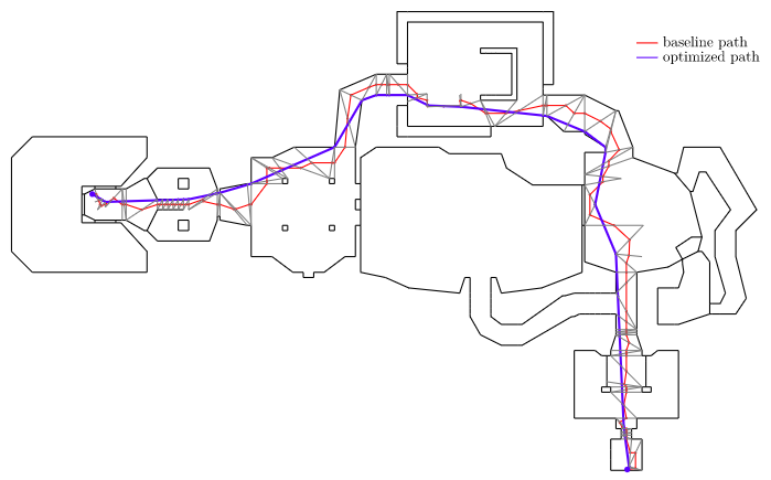
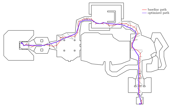
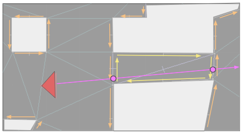
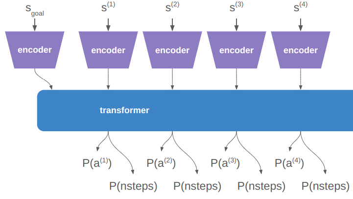
In a previous post, I had covered a project in which I was trying to get a neural network to learn to play Sokoban. I trained a transformer that operated on encoded board positions and predicted both the next action and how many steps were left until a solution would be reached:
My training was all done with Flux.jl and my own transformer implementation, not because it was more efficient or anything, but because I like to learn by doing it myself.
This training all happened on my little personal laptop. I love my laptop, but it is not particularly beefy, and it does not have much of a GPU to speak of. Training a fairly simple transformer was taking a long time — around 8 hours — which is pretty long. That doesn’t leave much room for experimentation. I knew that all this training was happening on the CPU, and the best way to make it faster would be to move to the GPU.
Flux making moving to the GPU incredibly easy:
using CUDA
policy = TransformerPolicy(
    batch_size = BATCH_SIZE,
    max_seq_len = MAX_SEQ_LEN,
    encoding_dim = ENCODING_DIM,
    dropout_prob=dropout_prob,
    no_past_info=no_past_info) |> gpu
That’s it – you just use the CUDA package and pipe your model to the GPU.
I tried this, and… it didn’t work. Unfortunately my little laptop does not have a CUDA-capable GPU.
After going through a saga of trying to get access to GPUs in AWS, I put the project to the side. There is sat, waiting for me to eventually pick it back up again whenever I ultimately decided to get a machine with a proper GPU or try to wrangle AWS again.
Then, one fateful day, I happened to be doing some cleaning and noticed an older laptop that I no longer used. Said laptop is bigger, and, just perhaps it had a CUDA-capable GPU. I booted it up, and lo and behold, it did. Not a particularly fancy graphics card, but CUDA-capable nonetheless.
This post is about how I used said GPU to train my Sokoban models, and how I then set up a task system in order to run a variety of parameterizations.
Model Training with a GPU
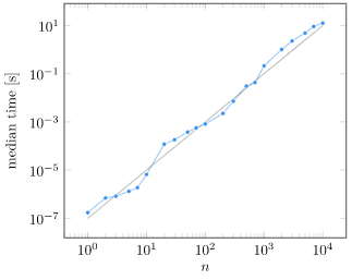
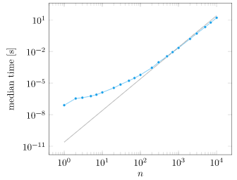
I switched my training code to move as much stuff as possible over to the GPU. After some elbow grease, I kicked off the same training run before and found that it ran in about 15 min – a 32x speed increase.
The next thing I tried was increasing the encoding from a length of 16 to 32. On the CPU, such an increase would at least double the training time. On the GPU, the training time remained the same.
How could that be?
Simply put, the GPU is really fast at crunching numbers, and the training runtime is dominated by using the CPU to unpack our training examples, sending data to and from the GPU, and running the gradient update on the CPU. In this case there seems to be a free lunch!
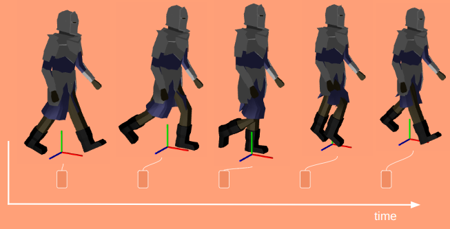
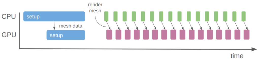
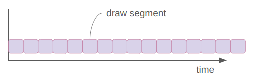
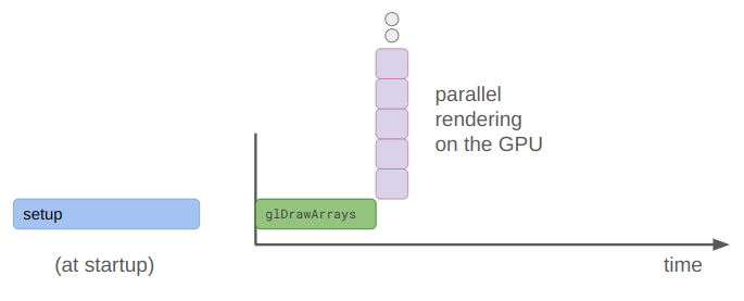
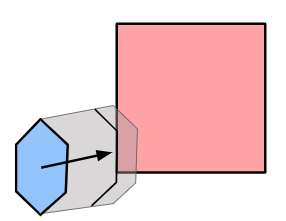
Here is a simple depiction of what was happening before (top timeline) vs. what is happening now:
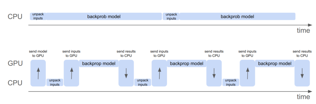
We pay the upfront cost of sending the model to the GPU, but then can more efficiently shovel data into it to get results faster than computing them ourselves. There is nothing magical happening here, just literally passing data there, having it crunch it, and receiving it once its done.
Parameter Tuning
Now that we have faster training, it is nice to look at how various training and model parameters affect our metrics. Good parameters can easily make or break a deep learning project.
Our model parameters are:
- board dimension – always \(8 \times 8\)
- encoding dimension – the size of the transformer embedding
- maximum sequence length – how long of a sequence the transformer can handle (always 64)
- number of transformer layers
Our training parameters are:
- learning rate – affects the size of the steps that our AdamW optimizer takes
- AdamW 1st and 2nd momentum decay
- AdamW weight decay
- batch size – the number of training samples per optimization step
- number of training batches – the number of optimization steps
- number of training entries – the size of our training set
- dropout probability – certain layers in the transformer have a chance of randomly dropping outputs for robustness purposes
- gradient threshold – the gradient is clipped to this value to improve stability
That’s a lot of parameters. How are we going to go about figuring out the best settings?
The tried and true method that happens in practice is try-and-see, where humans just try things they think are reasonable and see how the model performs. That’s what I was doing originally, when each training run took 8 hours. While that’s okay, it’d be nice to do better.
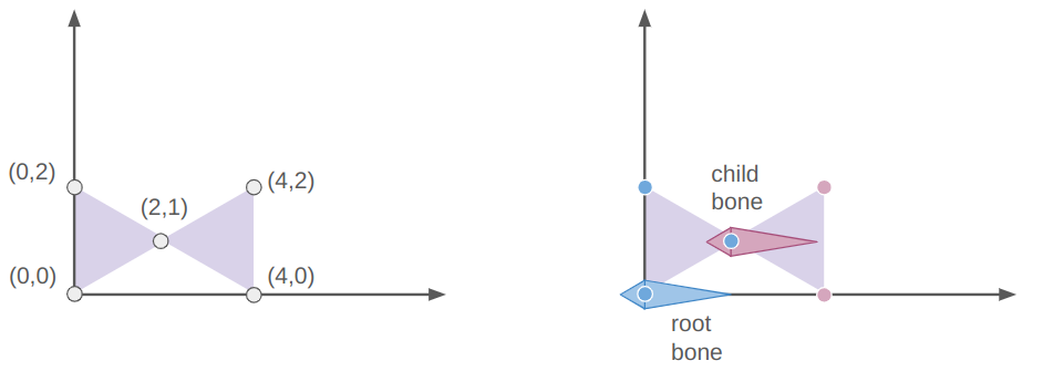
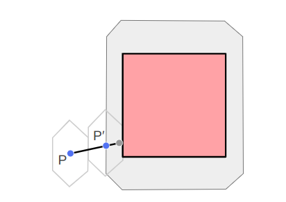
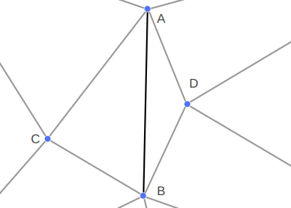
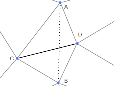
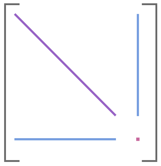
The next simplest approach is grid search. Here we discretize all parameters and train a model on every possible parameter combination. In 2 dimensions this ends up looking like a grid, hence the name:
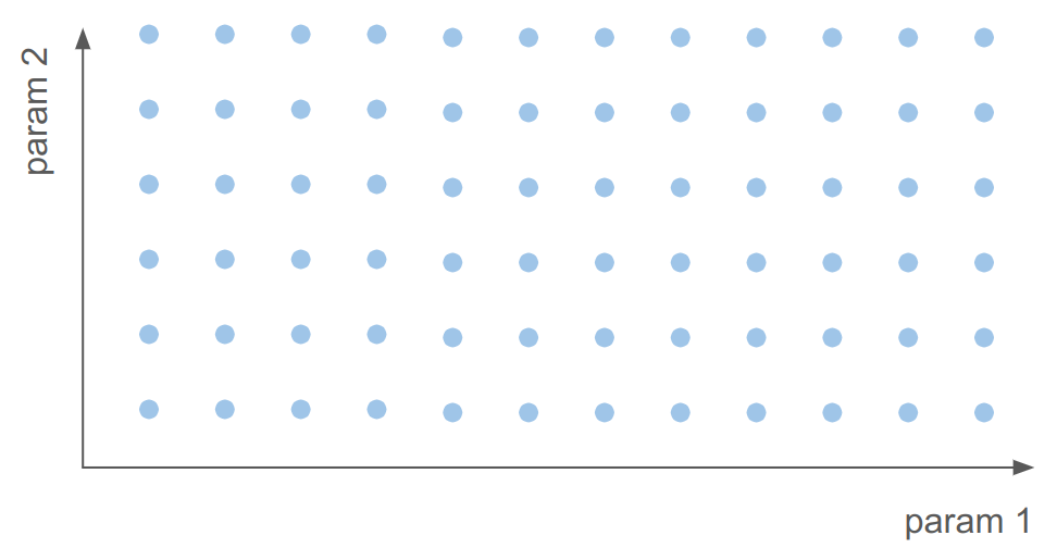
We have about 10 parameters. Even if we only consider 2 values for each of them, doing a grid search over them all would require training \(2^{10} = 1024\) models, which at 15 min per model is ~10.7 days. That’s both too long and pretty useless – we want higher granularity than that.
With grid search out, the next alternative is to conduct local searches for specific parameters. We already have a training parameterization that works pretty well, the one from the last blog post, and we can vary a single parameter and see how that affects training. That’s much cheaper – just the cost of the number of training points we’d like to evaluate per parameter. If we want to evaluate 5 values per parameter, that’s just \(5 \cdot 10 = 50\) models, or ~12.5 hours of training time. I could kick that off and come back to look at it the next day.
What I just proposed is very similar to cyclic coordinate search or coordinate descent, which is an optimization approach that optimizes one input at a time. It is quite simple, and actually works quite well. In fact, Sebastian Thrun himself has expressed his enthusiasm for this method to me.
There’s a whole realm of more complicated sampling strategies that could be followed. I rather like uniform projection plans and quasi-random space-filling sets like the Halton sequence. They don’t take that much effort to set up and do their best to fill the search space with a limited number of samples.
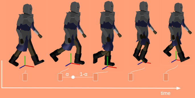
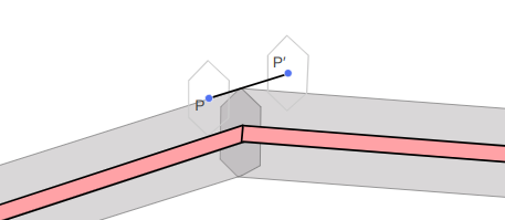
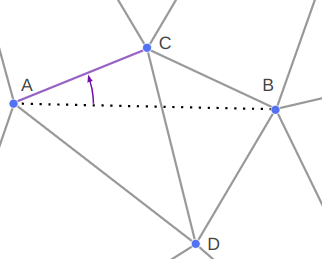
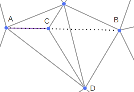
The method I most leaned up was ultimately a mixture of coordinate search and random sampling. Random sampling is what Andrej Karpathy recommended in CS231n, because it lets you evaluate far more independent values for specific parameters than something like grid search:
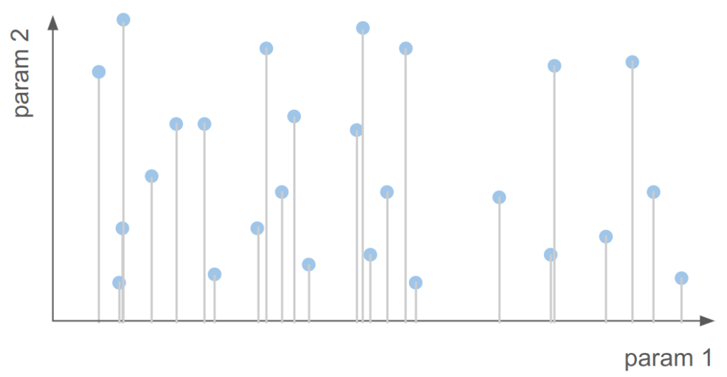
Here we see about 1/3 as many samples as grid search covering way more unique values for param 1.
Okay, so we want a way to run random search and perhaps some other, more targeted search approaches. How would we go about doing that?
Tasks
In the next phase of my project I want to expand from just training a transformer policy to predict player up/down/left/right moves to more complicated models that may interact with this simpler model. I also want to use my models to discover solutions to random problems, and perhaps refine previously discovered solutions with better models. I thus don’t want to merely support training this one model, I want to be able to run more general tasks.
function run_tasks()

    done = false
    while !done

        task_file = get_next_task()
        if !isa(task_file, String)
            println("No tasks left!")
            done = true
            break
        end

        task_filepath = joinpath(FOLDER_TODO, task_file::String)
        res = run_task(task_filepath)
        dest_folder = res.succeeded ? FOLDER_DONE : FOLDER_TRIED

        # name the task according to the time
        task_dst_name = Dates.format(Dates.now(), "yyyymmdd_HHMMss") * ".task"
        mv(task_filepath, joinpath(dest_folder, task_dst_name))
        write_out_result(res, task_dst_name, dest_folder)
        println(res.succeeded ? "SUCCEEDED" : "FAILED")
    end
end
The task runner simply looks for its next task in the TODO folder, executes it, and when it is done either moves it to the DONE folder or the TRIED folder. It then writes out additional task text that it captured (which can contain errors that are useful for debugging failed tasks).
The task runner is its own Julia process, and it spawns a new Julia process for every task. This helps ensure that issues in a task don’t pollute other tasks. I don’t want an early segfault to waste an entire night’s worth of training time.
The task files are simply Julia files that I load and prepend with a common header:
function run_task(task_filepath::AbstractString)
    res = TaskResult(false, "", time(), NaN)

    try
        content = read(task_filepath, String)

        temp_file, temp_io = mktemp()
        write(temp_io, TASK_HEADER)
        write(temp_io, "\n")
        write(temp_io, content)
        close(temp_io)

        output = read(`julia -q $(temp_file)`, String)

        res.succeeded = true
        res.message = output
    catch e
        # We failed to
        res.succeeded = false
        res.message = string(e)
    end

    res.t_elapsed = time() - res.t_start

    return res
end
This setup is quite nice. I can drop new task files in and the task runner with just dutifully run them as soon as its done with whatever came before. I can inspect the TRIED folder for failed tasks and look at the output for what went wrong.
Results
I ran a bunch of training runs and then loaded and plotted the results to get some insight. Let’s take a look and see if we learn anything.
We’ve got a bunch of metrics, but I’m primarily concerned with the top-2 policy accuracy and the top-2 nsteps accuracy. Both of these measure how often the policy had the correct action (policy accuracy) or number of steps remaining (nsteps accuracy) in its top-2 most likely predictions. The bigger these numbers are the better, with optimal performance being 1.0.
First let’s look at the learning rate, the main parameter that everyone typically has to futz with. First, the top-2 policy accuracy:
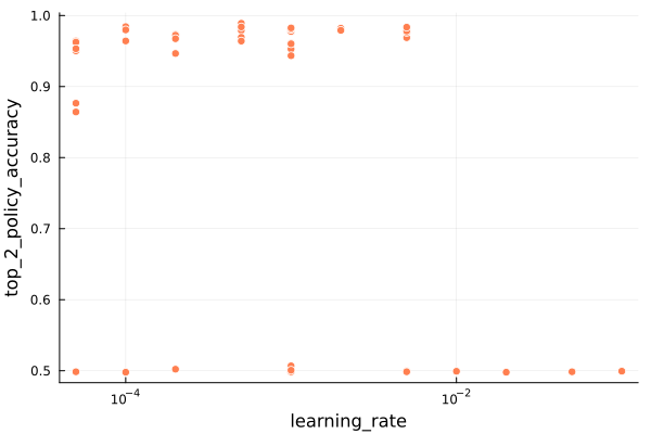
We immediately see a clear division between training runs with terrible accuracies (50%) and training runs with reasonable performance. This tells us that some of our model training runs did pretty poorly. That’s good to know – the parameters very much matter and can totally derail training.
Let’s zoom in on the good results:
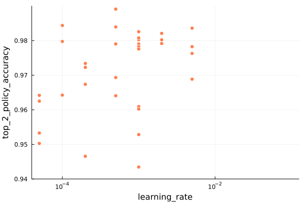
We don’t see a super-clear trend in learning rate. The best policy accuracy was obtained with a learning rate around 5e-4, but that one sample is somewhat of an outlier.
The nsteps accuracy also shows the bad models, so we’ll jump straight to the zoomed version:
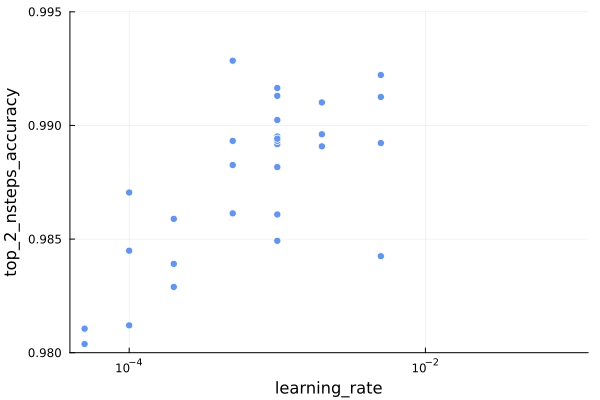
Interestingly, the same learning rate of 5e-4 produces the best nsteps accuracy as well, which is nice for us. Also, the overall spread here tends to prefer larger learning rates, with values down at 1e-4 trending markedly worse.
Next let’s look at the dropout probability. Large enough values are sure to tank training performance, but when does that start happening?
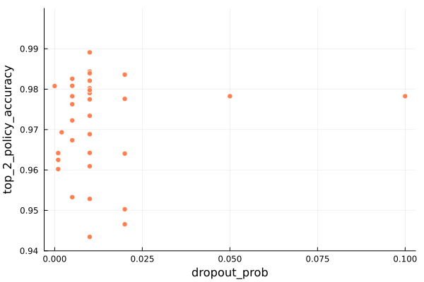
We don’t really have great coverage on the upper end, but based on the samples here it seems that a dropout probability of about 0.01 (or 1%) performs best. The nsteps accuracy shows a similar result.
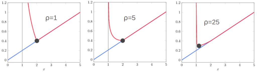
Next let’s look at the weight decay.
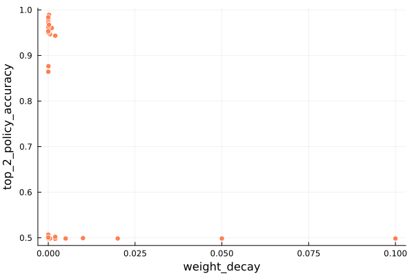
We’ve found our performance-tanking culprit! Weight decay values even moderately larger than zero appear to be highly correlated with terrible performance. It seems to drag the model down and prevent learning. Very small weight decay values appear to be fine, so we’ll have to be careful to just search those.
This is an important aspect of parameter tuning – parameters like the learning rate or weight decay can take on rather small values like 1e-4. Its often more about finding the right exponent rather than finding the right decimal value.
With those learning parameters out of the way, let’s look at some model parameters. First, the encoding dimension:
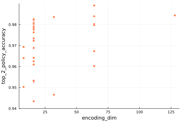
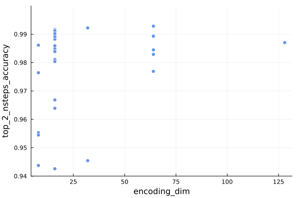
Naively we would expect that bigger encoding dimensions would be better given infinite training examples and compute, but we those are finite. We didn’t exhaustively evaluate larger encoding dimensions, but find that the nsteps prediction doesn’t benefit all that much from going from 32 to 64 entries, whereas the policy does.
We can also look at the number of transformer layers:
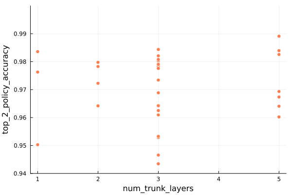
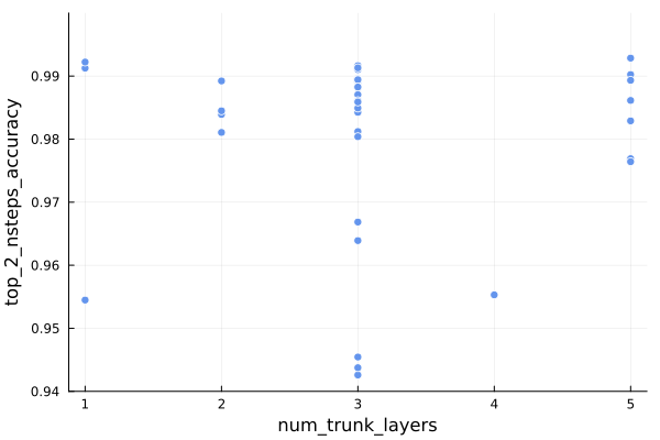
Having more layers means we have a bigger model, with more room to perform operations on our token embeddings as they pass through the model. Bigger is often better, but is ultimately constrained by our training data and compute.
In this case the nsteps predictor can achieve peak performance across a variety of depths, whereas the policy seems to favor larger layer counts (but can still do pretty well even with a single layer).
The next question we might ask is whether the mode size overall is predictive of performance. We can plot the total number of trainable parameters:
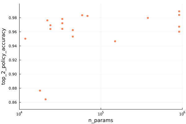
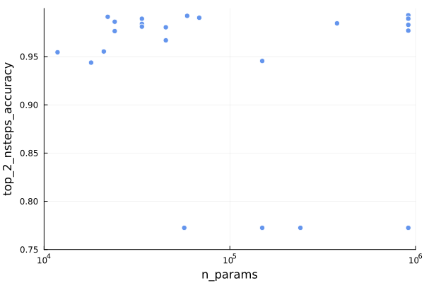
In terms of policy accuracy, we are seeing the best performance with the largest models, but the nsteps predictor doesn’t seem to need it as much. That is consistent with what we’ve already observed.
Let’s now identify the best model. How would we do that?
I’m going to consider the best model to be the one with the highest value of top-2 policy accuracy + top-2 nsteps accuracy. That’s the same as asking for the model most top-right in the following plot:
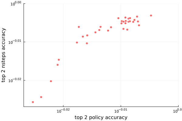
The two accuracies are highly correlated (which makes sense – its hard to predict how many steps it will take to reach the goal without also being a good Sokoban policy). The model that does the best has an encoding dim of 64 with 5 transformer layers, uses a learning rate of 0.0005, has weight decay = 0.0002, and a dropout probability of 0.01.
Conclusion
In this post I got excited about our ability to use the GPU to train our networks, and then I tried to capitalize on it by running a generic task runner. I did some sampling and collected a bunch of metrics in order to try to learn a thing or two about how best to parameterize my model and select the training hyperparameters.
Overall, I would say that the main takeaways are:
- Its worth spending a little time to help the computer do more work for you
- Its important to build insight into how the various parameters affect training
That’s all folks. Happy coding.