I spent a good while translating portions of the YASS Pascal code into Julia. I wanted to see how a larger, more sophisticated Sokoban solver works.
YASS (Yet Another Sokoban Solver), by Brian Damgaard, touts the use of a packing order calculation. I spent many hours trying to figure out what this was, and in the end boiled down the fundamental idea: it is a macro search where, instead of using individual box moves, the actions consist of either pushing a box all the way to a goal tile, or pushing a box as far away from its current position as possible with the hope that that frees up space for other boxes. That’s it.
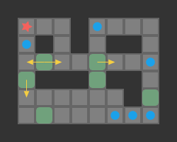
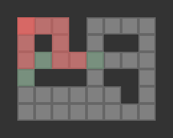
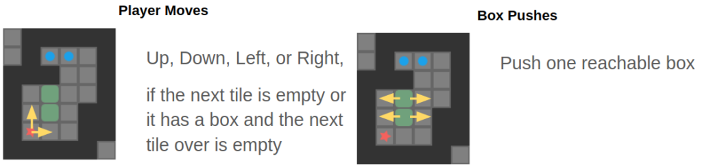
Sokoban solvers typically reason about individual pushes. Above we show the legal pushes for the current game state.
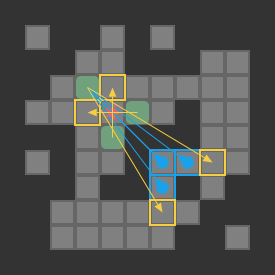
The macro actions available from the start state. These actions allow us to push a box to a goal (as shown with the right box) or to two possible farthest-away tiles.
The devil, of course, is in the details. YASS has a lot of additional bells and whistles, such as using deadlock sets and a special phase in which a box comes from a relatively small area of the board. This post merely looks at the core idea.
A Coarser Problem Representation
As mentioned above, most Sokoban solvers reason about pushes. This is already a coarser problem representation than basic Sokoban, where the actions are individual player moves. The coarser representation significantly reduces the size of the search tree. The player can move in four directions, so by collapsing ten moves that lead to a box push we can nicely remove O(4^10) possible states in our search tree.
Generally speaking, reasoning with a coarser problem representation lets us tackle larger problems. The larger, “chunkier” actions let us get more done with less consideration. The trade-off is that we give up fine-tune adjustments. When it comes to player moves vs. box pushes this is often well worth it. For the macro moves in packing order calculations, that is less true. (More on that later).
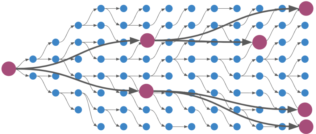
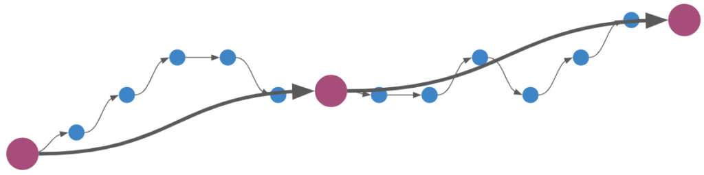
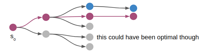
A notional image showing search with a high-fidelity representation (blue, ex: player moves) versus search with a coarse representation (magenta, ex: push moves).
If we solve a problem in a coarser representation, we need to be able to transform it back into the finer representation:
We need to be able to transform from macro actions back to our finer representation.
Transforming box pushes back into player moves is easy, as we simply find the shortest path for the player to the appropriate side of the box, and then tack on the additional step to push the box. In this case, we have a well-defined way to find the (locally) optimal sequence of player moves in order to complete the push.
The macro actions taken in the pure version of the packing order calculation I implemented work the same way. We simply calculate the push distance between tiles and find the shortest push path to the destination tile. As such, packing order macro actions are converted to pushes, which in turn can be converted to player moves.
Packing Order Search
Search problems are defined by their states, actions, and goalsand sometimes reward. Our coarser problem for packing order search is:
States – the same as Sokoban, augmented with an additional state for each box. For each box, we keep track of whether it is:
unmoved
temporarily parked
permanently parked
Actions:
An unmoved box can either be temporarily parked or pushed all the way to a goal, assuming the destination is reachable only by pushing that box.
A temporarily parked box can be pushed all the way to a goal, assuming the destination is reachable only by pushing that box. (It cannot be temporarily re-parked.)
YASS computes up to two candidate temporary parking tiles for each box:
the farthest tile in Manhattan distance from the box’s current position
the farthest tile in push distance from the box’s current position
Goals – the same as Sokoban. All boxes on goals.
Several things are immediately apparent. First, we can bound the size of our search tree. Every box can be moved at most twice. As such, if we have b boxes, then we can have at most 2^b macro actions. This in turn makes it obvious that not every problem can be solved with this search method. The search method, as is, is incomplete. Many Sokoban problems require moving a single box multiple times before bringing it to a goal. We could counteract that by allowing multiple re-parks, but we quickly grow our search tree if we do so.
The number of actions in a particular state is fairly large. A single box can be pushed to every goal it can reach, and can be parked on up to two possible candidate tiles. Since the number of goals is the same as the number of boxes, this means we have up to (2+b)^b actions in a single state. (Typically far less than that). As such, our tree is potentially quite fanned out. (In comparison, solving for box pushes has at most 4b actions in a single state).
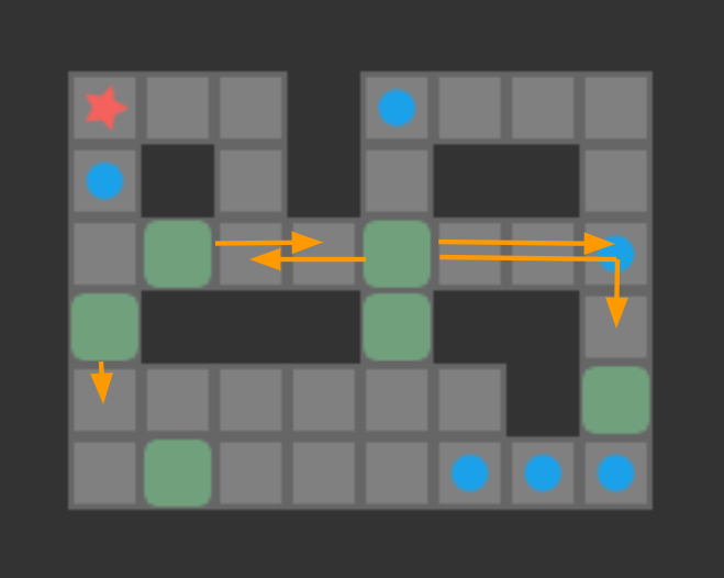
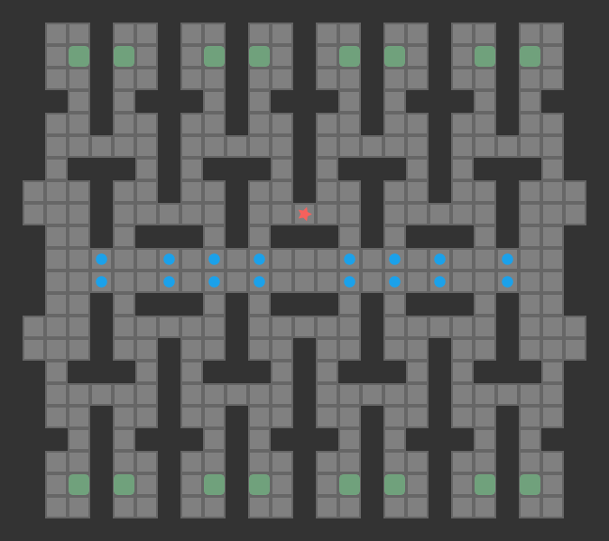
Here we see how the two lower-right boxes each only have one stashing location, but the upper-left box can be pushed to any goal or stashed next to the goals. (Note that we do not stash boxes in tiles from which they cannot be retrieved.)
We can apply pretty much any of the basic search algorithms from my previous post to this coarser problem representation. I just went with a basic depth-first search.
Below we can see a solution for a basic 3-box problem, along with its backed-out higher-fidelity versions:
Macro ActionsBox PushesPlayer Moves
While illustrative and a neat experience, this basic depth-first packing order search is not particularly great at solving Sokoban problems. It does, however, nicely illustrate the idea of translating between problem representations.
Reverse Packing Order Search
The packing order calculation done by YASS performs its search in reverse. That is, rather than starting with the initial board state and trying to push boxes to goals, it starts with all boxes on goals and tries to pull them to their starting states.
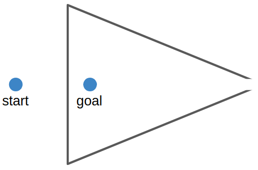
Reverse search and its various forms (ex: bidirectional search), are motivated by the fact that searching in the forward direction alone may not be as easy as the reverse direction. One common example is a continuous-space path finding problem in which the search has to find a way through a directional bottleneck:
A search from the start to the goal would likely have trouble to finding its way through the narrow opening, whereas a search from the goal to the start can be nicely funneled out.
The motivation for a reverse search in Sokoban is similar. However, rather than having to thread the needle through directional bottlenecks, Sokoban search has to avoid deadlock states. Reverse search is motivated by the idea that it is easier to get yourself into a deadlock state by pushing boxes than it is to get yourself into deadlock states by pulling boxes. This technique is presented in this paper by Frank Takes. Note that deadlocks are still possible – they just occur less frequently. That being said, 2×2 deadlocks won’t occur, the box cannot be pulled up against a wall or in a corner, etc.
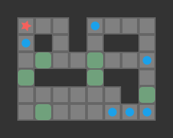
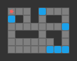
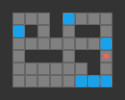
The starting state in a reverse search is a goal state – all boxes on goals. Note that we do not know where the player should start – they would end up next to one of the boxes. As such, we have to consider all player-reachable regions surrounding the goals. Below we show the initial state for a problem and three possible reverse search start states:
Original Start StateReverse Start State 1Reverse Start State 2Reverse Start State 3
My simple solver simply tries each possible start state until it finds a solution (or fails after exhausting all possibilities).
Reverse packing order search does perform betterAs measured by how many puzzles it can solve in 10s each on a test set than packing order search. It still suffers from incompleteness, and would need to be fleshed out with more bells and whistles to be useful (deadlock analysis, goal room packing, etc.). That being said, we can solve some problems that are too big for my previous version of A*, such as Sasquatch 49. We solve it in 0.002s.
Macro Actions (Pulls)
The push solution backed out from the macro-pull solution.
The player-move solution.
So there you have it, a simple solver that can handle an 8-box problem. Granted, it cannot solve most 8-box problems, but we have blazed a bit of a trail forward.
The main takeaway here is that one of the best ways to scale to larger problems is to reason with a coarser problem representation. We don’t plan every footstep when deciding to walk to the kitchen. Similarly, we reason about overall street routes when planning to drive somewhere, rather than thinking about every lane change (usually). Multi-level planning can be incredibly powerful – we just have to be careful to be able to back out feasible solutions, and not miss important details.
My last few blog posts covered methods for getting push-optimal solutions to simple Sokoban puzzles. Traditional Sokoban, however, operates on player moves. Solvers often reason about pushes to simplify decision-making. Unfortunately, push-optimal solutions are not necessarily move-optimal. For example, this solution is push-optimal but has some very clear inefficiencies when we render out the player moves required to travel between boxes:
Push-Optimal (but not move-optimal) solution for a subset of Sokoban 01
Rendering the same push-optimal solution above with its player moves clearly shows how inefficient it is
Directly solving for move-optimal solutions from scratch is difficult. Rather than doing that, it is common to optimize a given solution to try to find another solution with a smaller player move count. Thus, Sokoban solvers typically find push-optimal solutions, or more commonly some valid solution, and Sokoban optimizers work with an existing solution to try and improve it.
There are many approaches for optimizing solutions. In this post, I’ll just cover some very basic approaches to improve my push-optimal solutions from the previous posts.
Solution Evaluation
Every optimization problem needs an objective function. Here, we are trying to find solutions with fewer player moves. As such, our objective function takes in a potential push sequence solution and evaluates both its validity (whether it is, in fact, a solution), and the number of player moves. The number of player moves is the number of box pushes plus the number of moves to walk to the appropriate location for each push.
All of the strategies I use here simply shuffle the pushes around. I do not change the pushes. As we’ll see, this basic assumption works pretty well for the problems at hand.
We thus have a simple constrained optimization problem – to minimize the number of player moves by permuting the pushes in a provided push-optimal solution subject to the constraint that we maintain solution integrity. We can easily evaluate a given push sequence for validity by playing the game through with that push sequence, which we have to do anyway to calculate the number of player moves.
Strategy 1: Consider all Neighboring Box Pairs
The simplest optimization strategy is to try permuting neighboring push pairs. We consider neighboring pairs because they are temporally close, and thus more likely to be a valid switch. Two pushes that are spread out a lot in time are likely to not be switchable – other pushes are more likely to have to happen in-between.
This strategy is extremely simple. Just iterate over all pushes, and if two neighboring pushes are for two different boxes, try swapping the push order and then evaluating the new push sequence to see if it solves the problem with a smaller move count. If it does, keep the new solution.
For example, if our push sequence, in terms of box pushes, is AAABBCCBAD, we would evaluate AABABCCBAD first, and it does not lead to an improvement, consider AAABCBCBAD next, etc.
Strategy 2: Consider all Neighboring Same-Box Sequences
The strategy above is decent for fine-tuning the final solution. However, by itself it is often unable to make big improvements.
Move-optimal solutions are often achieved by grouping pushes for the same box together. This intuitively leads to the player not having to trek to other boxes between pushes – they are already right next to the box they need to push next. We thus can do quite well by considering moving chunks of pushes for the same box around rather than moving around a single box push at a time.
This approach scans through our pushes, and every time we change which box we are pushing, considers moving forward all push sequences of all other next boxes to before the current sequence of box pushes. For example, if our push sequence is AAABBCCBAD, we would consider BBAAACCBAD, CCAAABBBAD, and DAAABBCCBA, greedily keeping the first one that improves our objective.
Strategy 3: Group Same-Box Push Sequences
The third basic strategy that I implemented moves box sub-sequences in addition to full box sequences in an effort to consolidate same-box push sequences. For each push, if the next push is not for the same box, we find the next push sequence for this box and try to move the largest possible sub-sequence for that box to immediately after our current push – i.e., chaining pushes.
For example, if our push sequence is AAABBCCBAD, we would consider AAAABBCCBD, and if that did not lead to an improvement, would consider AAABBBCCAD.
Similarly, if our push sequence is AAABBAAA, we would consider AAAAAABB, then AAAAABBA, and finally AAAABBAA in an effort to find the largest sub-sequence we could consolidate.
Putting it All Together
None of these heuristics are particularly sophisticated or fancy. However, together we get some nice improvements. We can see the improvement on the full Sokoban 01 problem:
Full Push-Optimal Solution for Sokoban 01: 97 box pushes and 636 player moves
After re-ordering the pushes we have 260 only player moves
The following output shows how the algorithm progressed:
So there you have a quick-and-dirty way to get some nicer solutions out of our push-optimal solutions. Other approaches will of course be needed once we have solutions that aren’t push-optimal, which we’ll get once we move onto problems that are too difficult to solve optimally. There we’ll have to do more than just permute the pushes around, but actually try changing our push sequence and refining our solution more generally.
In my previous post, I covered some basic Sokoban search algorithms and some learnings from my digging into YASS (Yet Another Sokoban Solver). I covered the problem representation but glossed over how we determine the pushes available to us in a given board state. In this post, I cover how we calculate that and then conduct into a bunch of little efficiency investigations.
A push-optimal solution to a Sokoban puzzle
Set of Actions
We are trying to find push-optimal solutions to Sokoban problems. That is, we are trying to get every box on a box in the fewest number of pushes possible. As such, the actions available to us each round are the set of pushes that our player can conduct from their present position:
The set of pushes the player (red star) can conduct from their present position
Our Sokoban solver will need to calculate the set of available pushes in every state. As such, we end up calculating the pushes a lot, and the more efficient we are at it, the faster we can conduct our search.
A push is valid if:
our player can reach a tile adjacent to the block from their current position
the tile opposite the player, on the other side of the block, is free
As such, player reachability is crucial to the push calculation.
Reachablity for the same game state as the previous image. Red tiles are player-reachable, and green tiles are reachable boxes.
Above we see the tiles reachable from the player’s position (red) and the boxes adjacent to player-reachable tiles. This view is effectively the output of our reachability calculation.
Efficient Reach Calculations
The set of reachable tiles can be found with a simple flood-fill starting from the player’s starting location. We don’t care about the shortest distance, just reachability, so this can be achieved with either a breadth-first or a depth-first traversal:
Naive Reach Calculation
Let’s look at a naive Julia implementation using depth-first traversal:
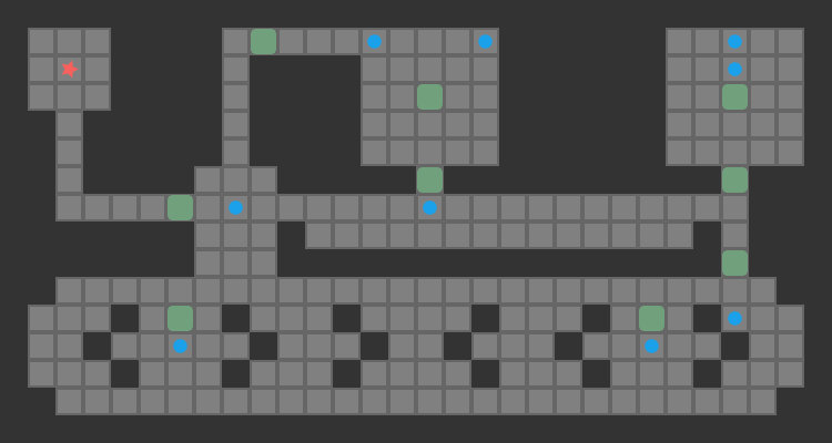
This code is somewhat inefficient, most notably in that it allocates sets for both reachable_tiles and reachable_boxes, which change in size during its execution. (We also compute the minimum reachable tile, for use in state hashing, as explained in the previous post.) Let’s evaluate its runtime on this large puzzle:
A large test puzzle based on Sasquatch 49. All tiles are initially reachable
Using @btime from BenchmarkTools.jl, we get 15.101 μs (28 allocations: 9.72 KiB). Honestly, 15 microseconds is actually quite good – much better than I expected from a naive implementation. That being said, let’s see if we can do better.
YASS Reach Calculation with Preallocated Memory
I spent a fair amount of time investigating YASS, which was written in Pascal. The Pascal code was structured differently than most of the code bases I’ve worked with. The working memory is declared and allocated at the top of the file in a global space, and is then used throughout. This preallocation makes it incredibly efficient. (As an aside, it was quite difficult to tell where variables were defined, since the naming conventions didn’t make it clear what was declared locally and what was global, and Pascal scoping really threw me into a loop). I feel that a lot of modern programming gets away with assuming we have a lot of memory, and is totally fine with paying the performance cost. However, in tight inner loops like this reach calculation, which might run many hundreds of thousands of times, we care enough about performance to pay special attention.
The Julia performance tips specifically call out paying attention to memory allocations. The previous code allocated 9.72 KiB. Let’s try to knock that down.
We’ll start by defining a struct that holds our preallocated memory. Rather than keeping lists or sets of player-reachable tiles and boxes, we’ll instead store a single flat array of tiles the same length as the board. This representation lets us just flag a given tile as a player-reachable tile or a player-reachable box:
mutable struct ReachableTiles
# The minimum (top-left) reachable tile. Used as a normalized player position
min_reachable_tile::TileIndex
# Incremented by 2 in each reach calculation# The player-reachable tiles have the value 'calc_counter'# Tiles with neighboring boxes have the value 'calc_counter' + 1# Non-floor tiles are set to typemax(UInt32)
calc_counter::UInt32
tiles::Vector{UInt32}end
This data structure lets us store everything we care about, and does not require clearing between calls (only once we get to wraparound). We just increment a counter and overwrite our memory with every call.
The reachability calculation from before can now be modified to update our ReachableTiles struct:
function calc_reachable_tiles!(
reach::ReachableTiles,
game::Game,
board::Board,
□_start::TileIndex,
stack::Vector{TileIndex})::Int# The calc counter wraps around when the upper bound is reachedif reach.calc_counter ≥ typemax(UInt32) - 2
clear!(reach, board)end
reach.calc_counter += 2
reach.min_reachable_tile = □_start
reach.tiles[□_start] = reach.calc_counter
n_reachable_tiles = 1# depth-first search uses a stackstack[1] = □_start
stack_hi = 1# index of most recently pushed item# stack contains items as long as stack_hi > 0while stack_hi >0# pop stack
□ = stack[stack_hi]
stack_hi -= 1# Examine tile neighborsfor dir in DIRECTIONS
▩ = □ + game.step_fore[dir]if reach.tiles[▩]< reach.calc_counter# An unvisited floor tile, possibly with a box# (non-floors are typemax ReachabilityCount)if(board[▩]& BOX) == 0# not a box
n_reachable_tiles += 1# push the square to the stack
stack_hi += 1stack[stack_hi] = ▩
reach.tiles[▩] = reach.calc_counter
reach.min_reachable_tile = min(▩, reach.min_reachable_tile)else# a box
reach.tiles[▩] = reach.calc_counter + 1endendendend
reach.calculated = truereturn n_reachable_tiles
end
This time, @btime gives us 2.490 μs (2 allocations: 224 bytes), which is about 6x faster and a massive reduction in allocations.
I was particularly pleased by the use of the stack memory passed into this method. Our depth-first traversal has to keep track of tiles that need to be expanded. The code uses a simple vector to store the stack, with just a single index variable stack_hi that points to the most recently pushed tile. We know that we will never have more items in the stack than tiles on our board, so stack can simply be the same length as our board. When we push, we increment stack_hi and place our item there. When we pop, we grab our item from stack[stack_hi] and then decrement. I loved the elegance of this when I discovered it. Nothing magic or anything, just satisfyingly clean and simple.
Avoiding Base.iterate
After memory allocations, the other thing common culprit of inefficient Julia code is a variable with an uncertain / wavering type. At the end of the day, everything ends up as assembly code that has to crunch real bytes in the CPU, so any variable that can be multiple things necessarily has to be treated in multiple ways, resulting in less efficient code.
Julia provides a @code_warntype macro that lets one look at a method to see if anything has a changing type. I ran it on the implementation above and was surprised to see an internal variable with a union type, @_9::Union{Nothing, Tuple{UInt8, UInt8}}.
It turns out that for dir in DIRECTIONS is calling Base.iterate, which returns either a tuple of the first item and initial state or nothing if empty. I was naively thinking that because DIRECTIONS was just 0x00:0x03 that this would be handled more efficiently. Anyways, I was able to avoid this call by using a while loop:
dir = DIR_UP
while dir <= DIR_RIGHT
    ...
    dir += 0x01
end
That change drops us down to 1.989 μs (2 allocations: 224 bytes), which is now about 7.5x faster than the original code. Not bad!
Graph-Based Board Representation
Finally, I wanted to try out a different board representation. The code about stores the board, a 2d grid, as a flat array. To move left we decrement our index, to move right we increment our index, and to move up or down we change by our row length.
I looked into changing the board to only store the non-wall tiles and represent it as a graph. That is, have a flat list of floor tiles and for every tile and every direction, store the index of its neighbor in that direction, or zero otherwise:
struct BoardGraph
# List of tile values, one for each node
tiles::Tiles
# Index of the tile neighbor for each tile.# A value of 0 means that edge is invalid.
neighbors::Matrix{TileIndex}# tile index × directionend
This form has the advantage of a smaller memory footprint. By dropping the wall tiles we can use about half the space. Traversal between tiles should be about as expensive as before.
The reach calculation looks more or less identical. As we’d expect, the performance is close to the same too: 2.314 μs (4 allocations: 256 bytes). There is some slight inefficiency, perhaps because memory lookup is not as predictable, but I don’t really know for sure. Evenly structured grid data is a nice thing!
Pushes
Once we’ve done our reachable tiles calculation, we need to use it to compute our pushes. The naive way is to just iterate over our boxes and append to a vector of pushes:
function get_pushes(game::Game, s::State, reach::ReachableTiles)
pushes = Push[]for(box_number, □)in enumerate(s.boxes)if is_reachable_box(□, reach)# Get a move for each direction we can get at it from,# provided that the opposing side is clear.for dir in DIRECTIONS
□_dest = □ + game.step_fore[dir]# Destination tile
□_player = □ - game.step_fore[dir]# Side of the player# If we can reach the player's pos and the destination is clear.if is_reachable(□_player, reach)&&((s.board[□_dest]&(FLOOR+BOX)) == FLOOR)push!(pushes, Push(box_number, dir))endendendendreturn pushes
end
We can of course modify this to use preallocated memory. In this case, we pass in a vector pushes. The most pushes we could have is four times the number of boxes. We allocate that much and have the method return the actual number of boxes:
function get_pushes!(pushes::Vector{Push}, game::Game, s::State, reach::ReachableTiles)::Int
n_pushes = 0for(box_number, □)in enumerate(s.boxes)if is_reachable_box(□, reach)# Get a move for each direction we can get at it from,# provided that the opposing side is clear.for dir in DIRECTIONS
□_dest = □ + game.step_fore[dir]# Destination tile
□_player = □ - game.step_fore[dir]# Side of the player# If we can reach the player's pos and the destination is clear.if is_reachable(□_player, reach)&&((s.board[□_dest]&(FLOOR+BOX)) == FLOOR)
n_pushes += 1
pushes[n_pushes] = Push(box_number, dir)endendendendreturn n_pushes
end
Easy! This lets us write solver code that looks like this:
An alternative is to do something similar to Base.iterate and generate the next push given the previous push:
"""
Given a push, produces the next valid push, with pushes ordered
by box_index and then by direction.
The first valid push can be obtained by passing in a box index of 1 and direction 0x00.
If there no valid next push, a push with box index 0 is returned.
"""function get_next_push!(
game::Game,
s::State,
reach::ReachableTiles,
push::Push = Push(1, 0))
box_index = push.box_index
dir = push.dirwhile box_index ≤ length(s.boxes)
□ = s.boxes[box_index]if is_reachable_box(□, reach)# Get a move for each direction we can get at it from,# provided that the opposing side is clear.while dir < N_DIRS
dir += one(Direction)
□_dest = game.board_start.neighbors[□, dir]
□_player = game.board_start.neighbors[□, OPPOSITE_DIRECTION[dir]]# If we can reach the player's pos and the destination is clear.if □_dest >0&&
□_player >0&&
is_reachable(□_player, reach)&&
not_set(s.tiles[□_dest], BOX)return Push(box_index, dir)endendend# Reset
dir = 0x00
box_index += one(BoxIndex)end# No next pushreturn Push(0, 0)end
We can then use it as follows, without the need to preallocate a list of pushes:
Both this code and the preallocated pushes approach are a little annoying, in a similar what that changing for dir in DIRECTIONS to a while loop is annoying. They uses up more lines than necessary and thus makes the code harder to read. That being said, these approaches are more efficient. Here are solve times using A* with all three methods on Sasquatch 02:
naive: 17.200 μs
Preallocated pushes: 16.480 μs
iterator: 15.049 μs
Conclusion
This post thoroughly covered how to compute the player-reachable tiles and player-reachable boxes for a given Sokoban board. Furthermore, we used this reachability to compute the valid pushes. We need the pushes in every state, so we end up computing both many times during a solver run.
I am surprised to say that my biggest takeaway is actually that premature optimization is the root of all evil. I had started this Sokoban project keen on figuring out how YASS could solve large Sokoban problems as effectively as possible. I spent a lot of time learning about its memory representations and using efficient preallocated memory implementations for the Julia solver.
I would never have guessed that the difference between a naive implementation and an optimized implementation for the reach calculation would merely yield a 7.5x improvement. Furthermore, I would never have thought that the naive implementation for getting the pushes would be basically the same as using a preallocated vector. There are improvements, yes, but it really goes to show that these improvements are really only worth it if you really measure your code and really need that speed boost. The sunk development time and the added code complexity is simply not worth it for a lot of everyday uses.
So far, the search algorithm used has had a far bigger impact on solver performance than memory allocation / code efficiencies. In some ways that makes me happy, as algorithms represent “how we go about something” and the memory allocation / efficiencies are more along the lines of implementation details.
As always, programmers need to use good judgement, and should look at objective data.
Sokoban – the basic block-pushing puzzle – has been on my mind off and on for several years now. Readers of my old blog know that I was working on a block-pushing video game for a short while back in 2012. John Blow, creator of The Witness, later announced that his next new game would draw a lot from Sokoban (In 2017? I don’t remember exactly). Back in 2018, when we were wrapping up Algorithms for Optimization and I started thinking about Algorithms for Decision Making, I had looked up some of the literature on Sokoban and learned about it more earnestly.
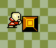
Mystic Dave pushing a block
At that time I stumbled upon Solving Sokoban by Timo Virkkala, a great Master’s Thesis that covers the basics of the game and the basics used by many solvers. The thesis serves as a great background for search in general, that is, whenever one wants to find the best sequence of deterministic transitions to some goal state. While search problems are not front and center in Algorithms for Decision Making, I did end up writing an appendix chapter on them, and looking back on it see how well comparatively the thesis covers the space.
I started work at Volley Automation in January of 2021, a startup working on fully automated parking garages. I am responsible for the scheduler, which is the centralized planner that orchestrates all garage operations. While the solo pushing of blocks in Sokoban is not quite the same as simultaneously moving multiple robots under trays and having them lift them up, the problems are fairly related. This renewed my interest in Sokoban, and I spent a fair amount of free time looking into solvers.
Early in my investigation, I downloaded an implementation of YASS (Yet Another Sokoban Solver), a 27538-line Pascal program principally written by Brian Damgaard, which I found via the Sokoban wiki. I had heard that this solver could solve the “XSokoban #50” level in under a second, and had found the wiki overview and the code, so felt it was a good place to dive in. After trying to translate the Pascal code into Julia directly, I both determined that the languages are sufficiently different that this was not really possible (Pascal, for example, has a construct similar to a C union, which Julia does not have), and that it also ultimately wasn’t what I wanted to get out of the exercise. I did learn a lot about Pascal and about efficient Sokoban solving from the code base, and ended up translating the overall gist of many algorithms in order to learn how Goal room packing works.
Before I fleshed out YASS’s goal room packing algorithm, I needed a good baseline and a way to verify that my Sokoban game code was correct. As such, I naturally started by writing some of the very basic search algorithms from my search appendix chapter. This post will cover these search algorithms and concretely show how they progressively improve on each other Sokoban problems of increasing complexity. It was really stark to see how the additions in each new algorithm causes order-of-magnitude changes in solver capability. As always, code is here.
Sokoban Basics
Sokoban is a search problem where a player is on a grid and needs to push some number of boxes to an equal number of goal tiles. The player can move north, south, east, or west, provided that they do not run into a wall or box tile. A player may push a box by moving into its space, provided that the box can move into the next space over. A simple 2-box Sokoban game and solution are shown below:
The red star indicates the player position, boxes are green when not on goals, and blue when on goals. The dark tiles are walls.
While the action space is technically the set of legal north/south/east/west player moves, it is more efficient to reason about push moves instead. That is, search algorithms will consider the pushes available from the player’s current position. This simplification yields massive speedups without losing much in terms of practicality. If a push is chosen, we can back out the minimum number of player moves to achieve the push by simply using a shortest-path solver.
Player move vs. box push problem formulations. Reasoning with a coarser representation has big performance implications.
A push-optimal solution may not be player move optimal – for example it may alternate between pushing two different boxes that the player has to traverse between – but it is nevertheless well worth reasoning about push moves. Here is the push-move solution for the same simple 2-box problem:
Sokoban is made tricky by the fact that there are deadlocks. We cannot push a box that ends up in a corner, for example. It is not always obvious when one has reached a state from which deadlock is inevitable. A big concern in most Sokoban solvers is figuring out how to efficiently disregard such parts of the search tree.
Problem Representation
A search problem is defined by a state space, an action space, a transition function, and a reward function. Sokoban falls into the category of shortest path problems, which are search problems that simply penalize each step and yield zero reward once a destination state is reached. As such, we are searching for the smallest number of steps to reach a goal state.
The board here has both static and dynamic elements. The presents of walls or goals, for example, does not change as the player moves. This unchanging information, including some precomputed values, are stored in a Game struct:
struct Game
board_height::Int32
board_width::Int32
board::Board # The original board used for solving, # (which has some precomputation / modification in the tile bit fields)# Is of length (Width+2)*(Height+2); the extra 2 is for a wall-filled border
start_player_tile::TileIndex
goals::Vector{TileIndex}# The goal tiles do not change# □ + step_fore[dir] gives the tile one step in the given direction from □
step_fore::SVector{N_DIRS, TileIndex}# □ + step_left[dir] is the same as □ + step_fore[rot_left(dir)]
step_left::SVector{N_DIRS, TileIndex}# □ + step_right[dir] is the same as □ + step_fore[rot_right(dir)]
step_right::SVector{N_DIRS, TileIndex}end
where TileIndex is just an Int32 index into a flat Board array of tiles. That is,
const TileIndex = Int32# The index of a tile on the board - i.e. a position on the boardconst TileValue = UInt32 # The contents of a board squareconst Board = Vector{TileValue}# Of length (Width+2)*(Height+2)
The 2D board is thus represented as a 1D array of tiles. Each tile is a bit field whose flags can be set to indicate various properties. The basic ones, as you’d expect, are:
I represented the dynamic state, what we affect as we take our actions, as follows:
mutable struct State
    player::TileIndex
    boxes::Vector{TileIndex}
    board::Board
end
You’ll notice that our dynamic state thus contains all wall and goal locations. This might seem wasteful but ends up being quite useful.
An action is a push:
struct Push
    box_number::BoxNumber
    dir::Direction
end
where BoxNumber refers to a unique index for every box assigned at the start. We can use this index to access a specific box in a state’s boxes field.
Taking an action is as simple as:
function move!(s::State, game::Game, a::Push)
□ = s.boxes[a.box_number]# where box starts
▩ = □ + game.step_fore[a.dir]# where box ends up
s.board[s.player]&= ~PLAYER # Clear the player
s.board[□]&= ~BOX # Clear the box
s.player = □ # Player ends up where the box is.
s.boxes[a.box_number] = ▩
s.board[s.player]|= PLAYER # Add the player
s.board[▩]|= BOX # Add the boxreturn s
end
Yeah, Julia supports unicode 🙂
Note that this method updates the state rather than producing a new state. It would certainly be possible to make it functional, but then we wouldn’t want to carry around our full board representation. YASS didn’t do this, and I didn’t want to either. That being said, in order to remain efficient we need a way to undo an action. This will let us efficiently backtrack when navigating up and down a search tree.
function unmove!(s::State, game::Game, a::Push)
□ = s.boxes[a.box_number]# where box starts
▩ = □ - game.step_fore[a.dir]# where box ends up
s.board[s.player]&= ~PLAYER # Clear the player
s.board[□]&= ~BOX # Clear the box
s.player = ▩ - game.step_fore[a.dir]# Player ends up behind the box.
s.boxes[a.box_number] = ▩
s.board[s.player]|= PLAYER # Add the player
s.board[▩]|= BOX # Add the boxreturn s
end
Finally, we need a way to know when we have reached a goal state. This is when every box is on a goal:
function is_solved(game::Game, s::State)for □ in s.boxesif(game.board[□]& GOAL) == 0returnfalseendendreturntrueend
The hardest part is computing the set of legal pushes. It isn’t all that hard, but involves a search from the current player position, and I will leave that for a future blog post. Just note that I use a reach struct for that, which will show up in subsequent code blocks.
Depth First Search
I started with depth first search, which is a very basic search algorithm that simply tries all combinations of moves up to a certain depth:
Depth-first traversal of the search tree. Note that we can visit the same state multiple times
In the book we call this algorithm forward search. The algorithm is fairly straightforward:
struct DepthFirstSearch
d_max::Intstack::Vector{TileIndex}# Memory used for reachability calcsend
mutable struct DepthFirstSearchData
solved::Bool
pushes::Vector{Push}# of length d_max
sol_depth::Int# number of pushes in the solutionendfunction solve_helper(
dfs::DepthFirstSearch,
data::DepthFirstSearchData,
game::Game,
s::State,
reach::ReachableTiles,
d::Int)if is_solved(game, s)
data.solved = true
data.sol_depth = d
returntrueendif d ≥ dfs.d_max# We exceeded our max depthreturnfalseend
calc_reachable_tiles!(reach, game, s.board, s.player, dfs.stack)forpushin get_pushes(game, s, reach)
move!(s, game, push)if solve_helper(dfs, data, game, s, reach, d+1)
data.pushes[d+1] = pushreturntrueend
unmove!(s, game, push)end# Failed to find a solutionreturnfalseendfunction solve(dfs::DepthFirstSearch, game::Game, s::State, reach::ReachableTiles)
t_start = time()
data = DepthFirstSearchData(false, Array{Push}(undef, dfs.d_max), 0)
solve_helper(dfs, data, game, s, reach, 0)return data
end
You’ll notice that I broke the implementation apart into a DepthFirstSearch struct, which contains the solver parameters and memory used while solving, a DepthFirstSearchData struct, which contains the data used while running the search and is returned with the solution, and a recursive solve_helper method that conducts the search. I use this approach for all subsequent methods. (Note that I am simplifying the code a bit too – my original code tracks some additional statistics in DepthFirstSearchData, such as the number of pushes evaluated.)
Depth first search is able to solve the simple problem shown above, and does so fairly quickly:
While this is good, the 2-box problem is well, rather easy. It struggles with a slightly harder problem:
Furthermore, depth first search does not necessarily return a solution with a minimum number of steps. It is perfectly happy to return as soon as a solution is found.
Notice that I do not cover breadth-first search. Unlike depth-first search, breadth-first search is guaranteed to find the shortest path. Why don’t we use that? Doesn’t breadth-first search have the same space complexity as depth-first search, since it is the same algorithm but with a queue instead of a stack?
I am glad you asked. It turns out that DFS and BFS do indeed have the same complexity, assuming that we store the full state in both the stack and the queue. You will notice that this implementation of DFS does not store the full state. Instead, we apply a small state delta (via move!) to advance our state, and then undo the move when we backtrack (via unmove!). This approach is more efficient, especially if the deltas are small and the overall state is large.
Iterative Deepening Depth First Search
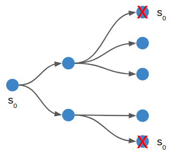
We can address the optimality issue by using iterative deepening. This is simply the act of running depth first search multiple times, each time increasing its maximum depth. We know that depth first search will find a solution if d_max is sufficiently large, and so the first run that finds a solution is guaranteed to be a minimum-push solution.
Depth-first search will return the first solution it finds. Here we show a solution (violet) at a deeper depth, when a shorter solution may still exist in an unexplored branch.
Notice that we evaluated more pushes by doing so, because we exhaustively search all 1-step search trees, all 2-step search trees, all 3-step search trees, …., all 7-step search trees before starting the 8-step search that found a solution. Now, the size of the search tree grows exponentially in depth, so this isn’t a huge cost hit, but nevertheless that explains the larger number for n_pushes_evaled.
Unfortunately, iterative deepening depth first search also chokes on the 3-box problem.
Zobrist Depth First Search
In order to tackle the 3-box problem, we need to avoid exhaustive searches. That is, depth first search will happily push a box left and then re-visit the previous state by pushing the box right again. We can save a lot of effort by not revising board states during a search.
We can save a lot of computational effort by not re-visiting states
The basic idea here is to use a transposition table to remember which states we have visited. We could simply store every state in that table, and only consider new states in the search if they aren’t already in our table.
Now, recall that our State struct is potentially rather large, and we are mutating it rather than producing a new one with every push. Storing all of those states in a table could quickly become prohibitively expensive. (Debatable, but this is certainly true for very large Sokoban problems).
One alternative to storing the full state is to store a hash value instead. The hash value, commonly a UInt64, takes up far less space. If a candidate state’s hash value is already in our transposition table, then we can be fairly confident that we have already visited it. (We cannot be perfectly confident, of course, because it is possible to get a hash collision, but we can be fairly confident nonetheless. If we’re very worried, we can increase the size of our hash to 128 bits or something).
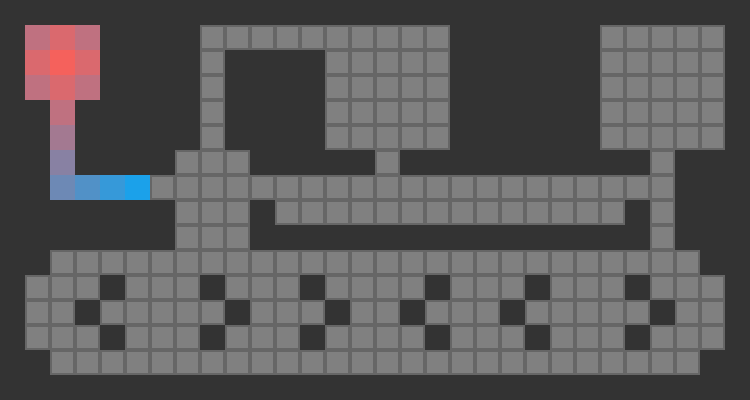
So to implement depth first search with a transposition table, we need a hash function. I learned a neat method from the YASS entry on the Sokoban wiki about how they do exactly this. First, we observe that the dynamic state that needs to be hashed is the player position and the box positions. Next, we observe that we don’t really care about the player position per-se, but rather which reachable region of the board the player is in. Consider the following game:
The player’s reachable space is:
As far as we are concerned, all of the highlighted tiles have the same legal pushes, so all states are equivalent when conducting a search.
We have to compute the player-reachable tiles anyhow when determining which pushes are legal. As such, we can “normalize” the player position in any state by just using the reachable tile with minimum index in board. If the box positions and this minimum player-reachable tile index match for two states, then we can consider them equivalent.
Finally, we need a way to hash the box positions. This is where Zobrist hashing comes in. This is a hashing technique that is commonly used in games like Sokoban and Chess because we can keep track of the hash by updating it with each move (and un-move), rather than having to recompute it every time from scratch. It works by associating a random unique UInt64 for every tile on the board, and we xor together all of the hash components that correspond to tiles with boxes on them:
function calculate_zobrist_hash(boxes::Vector{TileIndex}, hash_components::Vector{UInt64})::UInt64
result = zero(UInt64)for □ in boxes
result ⊻= hash_components[□]endreturn result
end
We can modify Game to store our Zobrist hash components.
The biggest win is that xor’s inverse is another xor. As such, we can modify State to include our current Zobrist hash, and we can modify move and unmove to simply apply and undo the xor:
function move!(s::State, game::Game, a::Push)
□ = s.boxes[a.box_number]
▩ = □ + game.step_fore[a.dir]
s.board[s.player]&= ~PLAYER
s.board[□]&= ~BOX
s.zhash ⊻= game.hash_components[□]# Undo the box's hash component
s.player = □
s.boxes[a.box_number] = ▩
s.board[s.player]|= PLAYER
s.board[▩]|= BOX
s.zhash ⊻= game.hash_components[▩]# Add the box's hash componentreturn s
end
Easy! Our algorithm is thus:
struct ZobristDFS
d_max::Intstack::Vector{TileIndex}# (player normalized pos, box zhash) → d_min
transposition_table::Dict{Tuple{TileIndex, UInt64},Int}end
mutable struct ZobristDFSData
solved::Bool
pushes::Vector{Push}# of length d_max
sol_depth::Int# number of pushes in the solutionendfunction solve_helper(
dfs::ZobristDFS,
data::ZobristDFSData,
game::Game,
s::State,
reach::ReachableTiles,
d::Int)if is_solved(game, s)
data.solved = true
data.sol_depth = d
returntrueendif d ≥ dfs.d_max# We exceeded our max depthreturnfalseend
calc_reachable_tiles!(reach, game, s.board, s.player, dfs.stack)# Set the position to the normalized location
s.player = reach.min_reachable_tile# Exit early if we have seen this state before at this shallow of a depth
ztup = (s.player, s.zhash)
d_seen = get(dfs.transposition_table, ztup, typemax(Int))if d_seen ≤ d
# Skip!
data.n_pushes_skipped += 1returnfalseend# Store this state hash in our transposition table
dfs.transposition_table[ztup] = d
forpushin get_pushes(game, s, reach)
data.n_pushes_evaled += 1
move!(s, game, push)if solve_helper(dfs, data, game, s, reach, d+1)
data.pushes[d+1] = pushreturntrueend
unmove!(s, game, push)end# Failed to find a solutionreturnfalseendfunction solve(dfs::ZobristDFS, game::Game, s::State, reach::ReachableTiles)
empty!(dfs.transposition_table)# Ensure we always start with an empty transposition table
data = ZobristDFSData(false, Array{Push}(undef, dfs.d_max), 0)
solve_helper(dfs, data, game, s, reach, 0)return data
end
This algorithm performs better on the 2-box problem:
Note how it evaluated 235522 pushes and did not find an optimal solution. We can combine the Zobrist hashing approach with iterative deepening to get an optimal solution:
A push-optimal solution for the 3-box problem. Notice that this is not player-move optimal.
A* (Best First Search)
For our next improvement, we are going to try to guide our search in the right direction. The previous methods are happy to try all possible ways to push a box, without any intelligence having it tend to push boxes toward a goal, for instance. We can often save a lot of computation by trying things that naively get us closer to our goal.
Where depth-first search expands our frontier in a depth-first order, A* (or best-first search), will expand our frontier in a best-first order. Doesn’t that sound good?
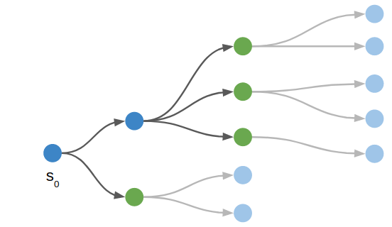
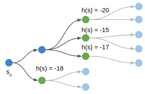
A* can expand any node in the frontier, and selects the node that it predicts has the best chance of efficiently reaching the goal
A*, pronounced “A Star”, is a best first search algorithm. It orders its actions according to how good the pushes are, where “goodness” is evaluated by a heuristic function. We are trying to minimize the number of pushes, and as long as this heuristic function gives as a lower bound on the true minimum number of pushes, A* will eventually find an optimal solution.
A* uses a heuristic function (plus the cost to reach a node) to evaluate each node in the frontier. It expands the node with the highest predicted reward (i.e., lowest cost).
As with Zobrist depth first search, A* also uses state hashes to know which states have been visited. Unlike Zobrist depth first search, A* maintains a priority queue over which state to try next. This presents a problem, because we don’t store states, but rather apply pushes in order to get from one state to another. Once again, YASS provided a nifty way to do something, this time to efficiently switch from states in one part of the search tree to another.
We will store a search tree for our visited states, but instead of each node storing the full state, we will instead store the push leading to the position. We can get from one state to another by traversing backwards to the states’ common ancestor and then traversing forwards to the destination state. I find the setup to be rather clever:
const PositionIndex = UInt32
mutable struct Position
pred::PositionIndex # predecessor index in positions arraypush::Push # the push leading to this position
push_depth::Int32# search depth
lowerbound::Int32# heuristic cost-to-go
on_path::Bool# whether this move is on the active search pathend
function set_position!(
s::State,
game::Game,
positions::Vector{Position},
dest_pos_index::PositionIndex,
curr_pos_index::PositionIndex,
)# Backtrack from the destination state until we find a common ancestor,# as indicated by `on_path`. We reverse the `pred` pointers as we go# so we can find our way back.
pos_index = dest_pos_index
next_pos_index = zero(PositionIndex)while(pos_index != 0)&&(!positions[pos_index].on_path)
temp = positions[pos_index].pred
positions[pos_index].pred = next_pos_index
next_pos_index = pos_index
pos_index = temp
end# Backtrack from the source state until we reach the common ancestor.while(curr_pos_index != pos_index)&&(curr_pos_index != 0)
positions[curr_pos_index].on_path = false
unmove!(s, game, positions[curr_pos_index].push)
curr_pos_index = positions[curr_pos_index].predend# Traverse up the tree to the destination state, reversing the pointers again.while next_pos_index != 0
move!(s, game, positions[next_pos_index].push)
positions[next_pos_index].on_path = true
temp = positions[next_pos_index].pred
positions[next_pos_index].pred = curr_pos_index
curr_pos_index = next_pos_index
next_pos_index = temp
endreturn s
end
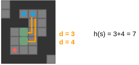
Our heuristic lower bound can take on many forms. One of the simplest is the sum of the distance of each box to the nearest goal, ignoring walls. This is definitely a lower bound, as we cannot possibly hope to require fewer pushes than that. Better lower bounds certainly exist – for example this lower bound does not take into account that each box must go to a different goal.
The lower bound we use is only slightly more fancy – we precompute the minimum number of pushes for each tile to the nearest goal ignoring other boxes, but not ignoring the walls. This allows us to recognize basic deadlock states where a box cannot possibly be moved to a goal, and it gives us a better lower bound when walls separate us from our goals.
Our cost lowerbound is the sum of the push distance of each box to the closest goal
The A* implementation is a little more involved than the previous algorithms, but its not too bad:
struct AStar
d_max::Int
n_positions::Intend
mutable struct AStarData
solved::Bool
max_depth::Int# max depth reached during search
pushes::Vector{Push}# of length d_max
sol_depth::Int# number of pushes in the solutionendfunction solve(solver::AStar, game::Game, s::State)
d_max, n_positions = solver.d_max, solver.n_positions# Allocate memory and recalculate some things
data = AStarData(false, Array{Push}(undef, d_max), 0)
reach = ReachableTiles(length(game.board))
clear!(reach, game.board)stack = Array{TileIndex}(undef, length(game.board))
pushes = Array{Push}(undef, 4*length(s.boxes))
queue_big = Array{Tuple{TileIndex, TileIndex, Int32}}(undef, length(s.board)* N_DIRS)
distances_by_direction = Array{Int32}(undef, length(s.board), N_DIRS)
dist_to_nearest_goal = zeros(Int32, length(s.board))
calc_push_dist_to_nearest_goal_for_all_squares!(dist_to_nearest_goal, game, s, reach, stack, queue_big, distances_by_direction)# Calculate reachability and set player min pos
calc_reachable_tiles!(reach, game, s.board, s.player, stack)
move_player!(s, reach.min_reachable_tile)# Compute the lower bound
simple_lower_bound = calculate_simple_lower_bound(s, dist_to_nearest_goal)# Allocate a bunch of positions
positions = Array{Position}(undef, n_positions)for i in1:length(positions)
positions[i] = Position(
zero(PositionIndex),
Push(0,0),
zero(Int32),
zero(Int32),
false)end# Index of the first free position# NOTE: For now we don't re-use positions
free_index = one(PositionIndex)# A priority queue used to order the states that we want to process,# in order by total cost (push_depth + lowerbound cost-to-go)
to_process = PriorityQueue{PositionIndex, Int32}()# A dictionary that maps (player pos, zhash) to position index,# representing the set of processed states
closed_set = Dict{Tuple{TileIndex, UInt64}, PositionIndex}()# Store an infeasible state in the first index# We point to this position any time we get an infeasible state
infeasible_state_index = free_index
positions[infeasible_state_index].lowerbound = typemax(Int32)
positions[infeasible_state_index].push_depth = zero(Int32)
free_index += one(PositionIndex)# Enqueue the root state
current_pos_index = zero(PositionIndex)
enqueue!(to_process, current_pos_index, simple_lower_bound)
closed_set[(s.player, s.zhash)] = current_pos_index
done = falsewhile!done&&!isempty(to_process)
pos_index = dequeue!(to_process)
set_position!(s, game, positions, pos_index, current_pos_index, data)
current_pos_index = pos_index
push_depth = pos_index >0? positions[pos_index].push_depth : zero(Int32)
calc_reachable_tiles!(reach, game, s.board, s.player, stack)# Iterate over pushes
n_pushes = get_pushes!(pushes, game, s, reach)for push_index in1:n_pushes
push = pushes[push_index]
move!(s, game, push)
calc_reachable_tiles!(reach, game, s.board, s.player, stack)
move_player!(s, reach.min_reachable_tile)# If we have not seen this state before so early, and it isn't an infeasible state
new_pos_index = get(closed_set, (s.player, s.zhash), zero(PositionIndex))if new_pos_index == 0|| push_depth+1< positions[new_pos_index].push_depth
lowerbound = calculate_simple_lower_bound(s, dist_to_nearest_goal)# Check to see if we are doneif lowerbound == 0# We are done!done = true# Back out the solution
data.solved = true
data.sol_depth = push_depth + 1
data.pushes[data.sol_depth] = push
pred = pos_index
while pred >0
pos = positions[pred]
data.pushes[pos.push_depth] = pos.push
pred = pos.predendbreakend# Enqueue and add to closed set if the lower bound indicates feasibilityif lowerbound != typemax(Int32)# Add the position
pos′ = positions[free_index]
pos′.pred = pos_index
pos′.push = push
pos′.push_depth = push_depth + 1
pos′.lowerbound = lowerbound
to_process[free_index] = pos′.push_depth + pos′.lowerbound
closed_set[(s.player, s.zhash)] = free_index
free_index += one(PositionIndex)else# Store infeasible state with a typemax index
data.n_infeasible_states += 1
closed_set[(s.player, s.zhash)] = infeasible_state_index
endelse
data.n_pushes_skipped += 1end
unmove!(s, game, push)endendreturn data
end
Notice that unlike the other algorithms, this one allocates a large set of positions for its search tree. If we use more positions than we’ve allocated, the algorithm fails. This added memory complexity is typically worth it though, as we’ll see.
It found an optimal solution by only evaluating 1,660 pushes, where iterative deepening Zobrist DFS evaluated 174,333. That is a massive win!
A* is able to solve the following 4-box puzzle to depth 38 by only evaluating 5,218 pushes, where iterative deepening Zobrist DFS evaluates 1,324,615:
A push-optimal solution for “Chaos”, a level by YASGen and Brian Damgaard
It turns out that A* can handle a few trickier puzzles:
Sasquatch 01
Sasquatch 02
However, it too fails as things get harder.
Conclusion
There you have it – four basic algorithms that progressively expand our capabilities at automatically solving Sokoban problems. Depth first search conducts a very basic exhaustive search to a maximum depth, iterative deepening allows us to find optimal solutions by progressively increasing our maximum depth, Zobrist hashing allows for an efficient means of managing a transposition table for Sokoban games, and A* with search tree traversal lets us expand the most promising moves.
The YASS codebase had plenty of more gems in it. For example, the author recognized that the lower bound + push depth we use in A* can only increase. As such, if we move a box toward a goal, our overall estimated cost stays the same. But, every state we move from is by definition a minimum-cost state, so the new state is also then minimum cost as well. We can thus save some computation by just continuing to expand from that new state. See, for example, the discussion in “Combining depth-first search with the open-list in A*“.
I’d like to cover the reachability calculation code in a future blog post. I thought it was a really good example of simple and efficient code design, and how the data structures we use influence how other code around it ends up being architected.
Thanks for reading!
Special thanks to Oscar Lindberg for corrective feedback on this post.