Convex duality is the sort of thing where you see the symbolic derivation and it sort of makes sense, but then you forget the steps and a day or two later you just sort of have to trust yourself that the theorems and facts hold but forget where they really come from. I recently relearned convex duality from the great lectures of Stephen Boyd, and in so doing, also learned about a neat geometry interpretation that helps solidify things.
Working with Infinite Steps
Everything starts with an optimization problem in standard form:
\[\begin{matrix}\underset{\boldsymbol{x}}{\text{minimize}} & f(\boldsymbol{x}) \\ \text{subject to} & \boldsymbol{g}(\boldsymbol{x}) \leq \boldsymbol{0} \\ & \boldsymbol{h}(\boldsymbol{x}) = \boldsymbol{0} \end{matrix}\]
This problem has an objective \(f(\boldsymbol{x})\), some number of inequality constraints \(\boldsymbol{g}(\boldsymbol{x}) \leq \boldsymbol{0}\), and some number of equality constraints \(\boldsymbol{h}(\boldsymbol{x}) = \boldsymbol{0}\).
Solving an unconstrained optimization problem often involves sampling the objective and using its gradient, or several local values, to know which direction to head in to find a better design \(\boldsymbol{x}\). Solving a constrained optimization problem isn’t as straightforward – we cannot accept a design that violates any constraints.
We can, however, view our constrained optimization problem as an unconstrained optimization problem. We simply incorporate our constraints into our objective, setting them to infinity when the constraints are violated and setting them to zero when the constraints are met:
\[\underset{\boldsymbol{x}}{\text{minimize}} \enspace f(\boldsymbol{x}) + \sum_i \infty \cdot \left( g_i(\boldsymbol{x}) > 0\right) + \sum_j \infty \cdot \left( h_j(\boldsymbol{x}) \neq 0\right)\]
For example, if our problem is
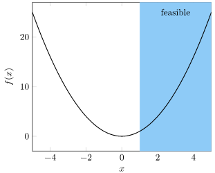
\[\begin{matrix}\underset{x}{\text{minimize}} & x^2 \\ \text{subject to} & x \geq 1 \end{matrix}\]
which looks like this
then we can rewrite it as
\[\underset{x}{\text{minimize}} \enspace x^2+\infty \cdot \left( x < 1\right)\]
which looks like
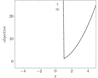
We’ve simply raised the value of infeasible points to infinity. Problem solved?
By doing this, we made our optimization problem much harder to solve with local methods. The gradient of designs in the infeasible region is zero, so we cannot use those to know which way to progress toward feasibility. It is also discontinuous. Furthermore, infinity is rather difficult to work with – it just produces more infinities when added or multiplied to most numbers. This new optimization problem is perhaps simpler, but we’ve lost a lot of information.
What we can do instead is reinterpret our objective slightly. What if, instead of using this infinite step, we simply multiplied our inequality function \(g(x) = 1 – x\) by a scalar \(\lambda\)?
\[\underset{x}{\text{minimize}} \enspace x^2+ \lambda \left( 1 – x \right)\]
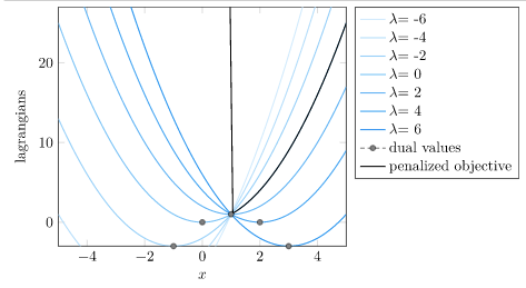
If we have a feasible \(x\), then \(\lambda = 0\) gives us the original objective function. If we have an infeasible \(x\), then \(\lambda = \infty\) gives us the penalized objective function.
We’re taking the objective and constraint, which are separate functions:
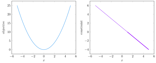
and combining them into a single objective based on \(\lambda\):
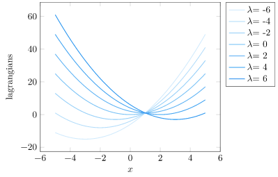
Let’s call our modified objective function the Lagrangian:
\[\mathcal{L}(x, \lambda) = x^2+ \lambda \left( 1 – x \right)\]
If we fix \(\lambda\), we can minimize our objective over \(x\). I am going to call these dual values:
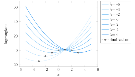
We find that all of these dual values are below the optimal value of the original problem:
This in itself is a big deal. We can produce a lower bound on the optimal value simply by minimizing the Lagrangian. Why is this?
Well, it turns out that we are guaranteed to get a lower bound any time that \(\lambda \geq 0\). This is because a positive \(\lambda\) ensures that our penalized objective is at or below the original objective for all feasible points. Minimizing is thus guaranteed to give us a design at or below the original value.
This is such a big deal, that we’ll call this minimization problem the Lagrange dual function, and give it a shorthand:
\[\mathcal{D}(\lambda) = \underset{x}{\text{minimize}} \enspace \mathcal{L}(x, \lambda)\]
which for our problem is
\[\mathcal{D}(\lambda) = \underset{x}{\text{minimize}} \enspace x^2 + \lambda \left( 1 – x \right)\]
Okay, so we have a way to get a lower bound. How about we get the *best* lower bound? That gives rise to the Lagrange dual problem:
\[\underset{\lambda \geq 0}{\text{maximize}} \enspace \mathcal{D}(\lambda)\]
For our example problem, the best lower bound is given by \(\lambda = 2\), which produces \(x = 1\), \(f(x) = 1\). This is the solution to the original problem.
Having access to a lower bound can be incredibly useful. It isn’t guaranteed to be useful (the lower bound can be \(-\infty\)), but it can also be relatively close to optimal. For convex problems, the bound is tight – the solution to the Lagrange dual problem has the same value as the solution to the original (primal) problem.
A Geometric Interpretation
We’ve been working with a lot of symbols. We have some plots, but I’d love to build further intuition with a geometric interpretation. This interpretation also comes from Boyd’s lectures, and textbook.
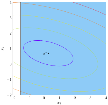
Let’s work with a slightly beefier optimization problem with a single inequality constraint:
\[\begin{matrix}\underset{\boldsymbol{x}}{\text{minimize}} & \|\boldsymbol{A} \boldsymbol{x} – \boldsymbol{b} \|_2^2 \\ \text{subject to} & x_1 \geq c \end{matrix}\]
In this case, I’ll use
\[\boldsymbol{A} = \begin{bmatrix} 1 & 0.3 \\ 0.3 & 2\end{bmatrix} \qquad \boldsymbol{b} = \begin{bmatrix} 0.5 \\ 1.5\end{bmatrix} \qquad c = 1.5\]
Let’s plot the objective, show the feasible set in blue, and show the optimal solution:
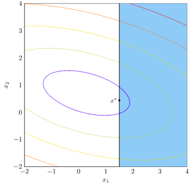
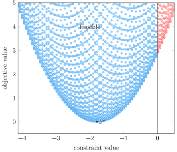
Our Lagrangian is again comprised of two terms – the objective function \( \|\boldsymbol{A} \boldsymbol{x} – \boldsymbol{b} \|_2^2\) and the constraint \(\lambda (c – x_1)\). We can build a neat geometric interpretation of convex duality by plotting (constraint, objective) pairs for various values of \(\boldsymbol{x}\):
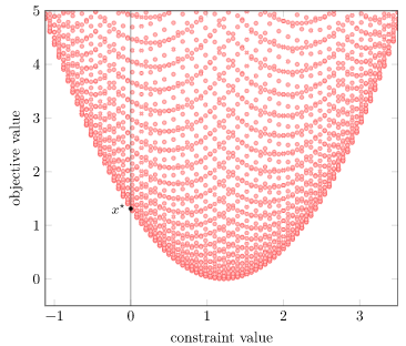
We get a parabolic region. This isn’t a huge surprise, given that we have a quadratic objective function.
Note that the horizontal axis is the constraint value. We only have feasibility when \(g(\boldsymbol{x}) \leq 0\), so our feasible designs are those left of the vertical line.
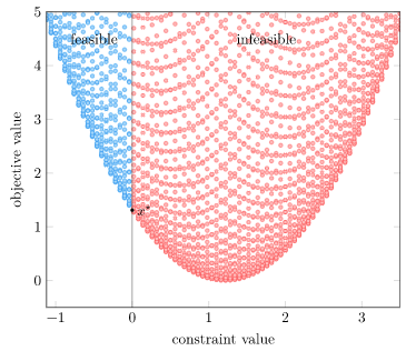
I’ve already plotted the optimal value – it is at the bottom of the feasible region. (Lower objective function values are better, and the bottom has the lowest value).
Let’s see if we can include our Lagrangian. The Lagrangian is:
\[\mathcal{L}(\boldsymbol{x}, \lambda) = f(\boldsymbol{x}) + \lambda g(\boldsymbol{x})\]
If we fix \(\boldsymbol{x}\), it is linear!
The Lagrange dual function is
\[\mathcal{D}(\lambda) = \underset{\boldsymbol{x}}{\text{minimize}} \enspace f(\boldsymbol{x}) + \lambda g(\boldsymbol{x})\]
If we evaluate \(\mathcal{D}\) for a particular \(\lambda\), we’ll minimize and get a design \(\hat{\boldsymbol{x}}\). The value of \(\mathcal{D}(\lambda)\) will be \(f(\hat{\boldsymbol{x}}) + \lambda g(\hat{\boldsymbol{x}})\). Remember, for \(\lambda \geq 0\) this is a lower bound. Said lower bound is the y-intercept of the line with slope \(-\lambda\) that passed through our (constraint, objective) at \(\hat{\boldsymbol{x}}\).
For example, with \(\lambda = 0.75\), we get:
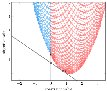
We got a lower bound, and it is indeed lower than the true optimum. Furthermore, that line is a supporting hyperplane of our feasible region.
Let’s try it again with \(\lambda = 3\):
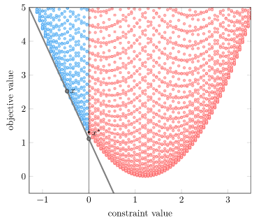
Our \(\lambda\) is still non-negative, so we get a valid lower bound. It is below our optimal value.
Now, in solving the Lagrange dual problem we get the best lower bound. This best lower bound just so happens to correspond to the \(\lambda\) that produces a supporting hyperplane at our optimum (\(\lambda \approx 2.15\)):
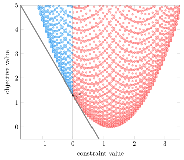
Our line is tangent at our optimum. This ties in nicely with the KKT conditions (out of scope for this blog post), which require that the gradient of the Lagrangian be zero at the optimum (for a problem with a differentiable objective and constraints), and thus the gradients of the objective and the constraints (weighted by \(\lambda\)) balance out.
Notice that in this case, the inequality constraint was active, with our optimum at the constraint boundary with \(g(\boldsymbol{x}) = 0\). We needed a positive \(\lambda\) to balance against the objective function gradient.
If we change our problem such that the unconstrained optimum is feasible, then we do not need a positive dual value to balance against the objective function gradient. Let’s adjust our constraint to max our solution feasible:
We now get an objective / constraint region with a minimum inside the feasible area:
Our best lower bound is obtained with \(\lambda = 0\):
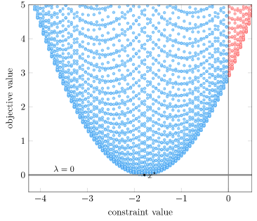
This demonstrates complementary slackness, the idea that \(\lambda_i g_i(\boldsymbol{x})\) is always zero. If constraint \(i\) is active, \(g_i(\boldsymbol{x}) = 0\);\ and if constraint \(i\) is inactive, \(\lambda_i = 0\).
So with this geometric interpretation, we can think of choosing \(\lambda\) as picking the slope of a line that supports this multidimensional volume from below and to the left. We want the line with the highest y-intercept.
Multiple Constraints (and Equality Constraints)
I started this post off with a problem with multiple inequality and equality constraints. In order to be thorough, I just wanted to mention that the Lagrangian and related concepts extend the way you’d expect:
\[\mathcal{L}(\boldsymbol{x}, \boldsymbol{\lambda}, \boldsymbol{\nu}) = f(\boldsymbol{x}) + \sum_i \lambda_i g_i(\boldsymbol{x}) + \sum_j \nu_j h_j(\boldsymbol{x})\]
and
\[\mathcal{D}(\boldsymbol{\lambda}, \boldsymbol{\nu}) = \underset{\boldsymbol{x}}{\text{maximize}} \enspace \mathcal{L}(\boldsymbol{x}, \boldsymbol{\lambda}, \boldsymbol{\nu})\]
We require that all \(\lambda\) values be nonnegative, but do not need to restrict the \(\nu\) values for the equality constraints. As such, our Lagrangian dual problem is:
\[\underset{\boldsymbol{\lambda} \geq \boldsymbol{0}, \>\boldsymbol{\nu}}{\text{maximize}} \enspace \mathcal{D}(\boldsymbol{\lambda}, \boldsymbol{\nu})\]
The geometric interpretation still holds – it just has more dimensions. We’re just finding supporting hyperplanes.