I recently started working on new chapters for Algorithms for Optimization, starting with a new chapter on quadratic programs. We already have a chapter on linear programs, but quadratic programs are sufficiently different and are ubiquitous enough that giving them their own chapter felt warranted.
The chapter starts with a general formulation for quadratic programs and transforms the problem a few times into simpler and simpler formulations, until we get a nonnegative least squares problem. This can be solved, and then we can use that solution to back our way up the transform stack back to a solution of our original solution.
In texts, these problem transforms are typically solely the realm of mathematical manipulations. While math is of course necessary, I also tried hard to depict what these various problem representations looked like to help build an intuitive understanding of what some of the transformations were. In particular, there was one figure where I wanted to show how the equality constraints of a general-form quadratic program could be removed when formulating a lower-dimensional least squares program:
This post is about this figure, and more specifically, about the blue contour lines on the left side.
What is this Figure?
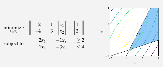
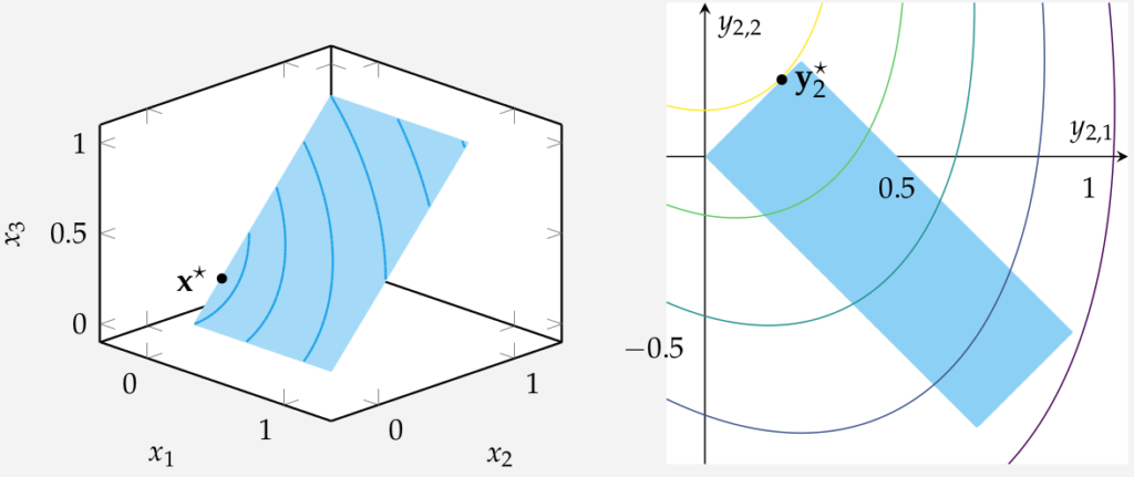
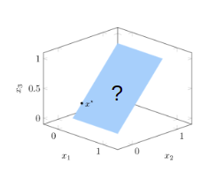
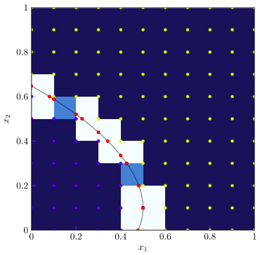
The figure on left shows the following quadratic program:
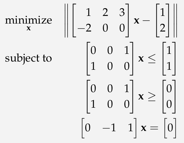
As we can see, the quadratic program is constrained to lie within a square planar region \(0 \leq x \leq 1\), \(0 \leq x_3 \leq 1\), and \(x_2 = x_3\). The feasible set is shown in blue.
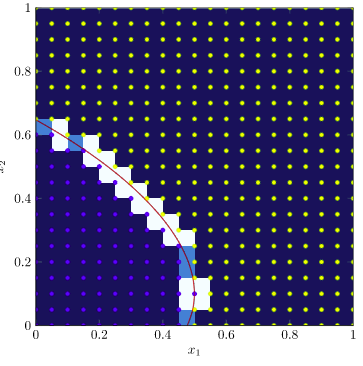
The right figure on the right shows the least-squares program that we get when we factor out the equality constraint. No need to get into the details here, it isn’t really important for this post, but we can use our one equality equation to remove one variable in our original problem, producing a 2d problem without any equality constraints:
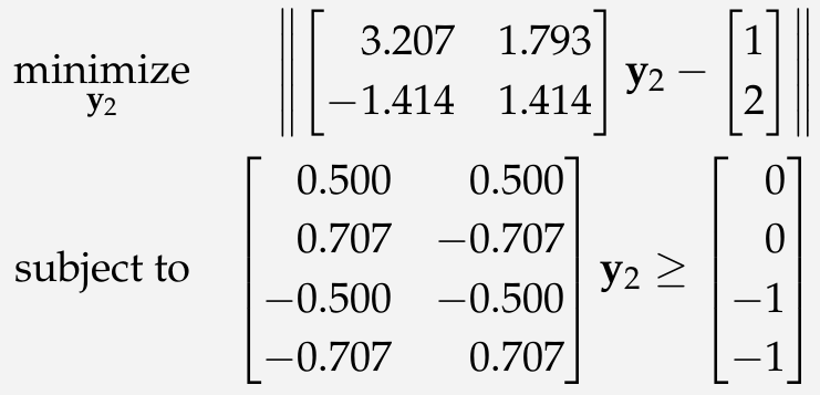
The original feasible set is rotated and stretched, and the objective function contours are rotated and stretched, but other than that we have a similar topology and a pretty standard problem that we can solve.
How do we Make the Figures?
I make the plots with PGFPlots.jl, which uses the pgfplots LaTeX package under the hood. It is a nice synergy of Julia coding and LaTeX within the LaTeX textbook.
Right Plot
The right plot is pretty straight forward. It has a contour plot for the objective function:
Plots.Contour(x -> norm(A_lsi*x - b_lsi, 2),
              xdomain, ydomain, xbins=600, ybins=600)
some over + under line plots and a fill-between for the feasible region:
x1_domain_feasible = (0.0, (0.5+√2)/2)
push!(plots,
      Plots.Linear(x1->max(-x1, x1 - sqrt(2)), x1_domain_feasible,
                   style="name path=A, draw=none, mark=none"))
push!(plots,
      Plots.Linear(x1->min(x1, 1/2-x1), x1_domain_feasible,
                   style="name path=B, draw=none, mark=none"))
push!(plots,
      Plots.Command("\\addplot[pastelBlue!50] fill between[of=A and B]"))
and a single-point scatter plot plus a label for the solution:
push!(plots,
      Plots.Scatter([x_val[1]], [x_val[2]],
      style="mark=*, mark size=1.25, mark options={solid, draw=black, fill=black}"))
push!(plots,
      Plots.Command("\\node at (axis cs:$(x_val[1]),$(x_val[2])) [anchor=west] {\\small \\textcolor{black}{\$y_2^\\star\$}}"))
These plots get added to an Axis and we’ve got our plot.
Left Plot
The left plot is in 3D. If we do away with the blue contour lines, its actually even simpler than the right plot. We simply have a square patch, a single-point scatter plot, and our label:
Axis([
   Plots.Command("\\addplot3[patch,patch type=rectangle, faceted color=none, color=pastelBlue!40] coordinates {(0,0,0) (1,0,0) (1,1,1) (0,1,1)}"),
   Plots.Linear3([x_val[1]], [x_val[2]], [x_val[3]], mark="*", style="mark size=1.1, only marks, mark options={draw=black, fill=black}"),
   Plots.Command("\\node at (axis cs:$(x_val[1]),$(x_val[2]),$(x_val[3])) [anchor=west] {\\small \\textcolor{black}{\$x^\\star\$}}"),
  ],
  xlabel=L"x_1", ylabel=L"x_2", zlabel=L"x_3", width="1.2*$width",
  style="view={45}{20}, axis equal",
  legendPos="outer north east"
)
The question is – how do we create that contour plot, and how do we get it to lie on that blue patch?
How do you Draw Contours?
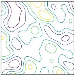
Contour plots don’t seem difficult to plot, until you have to sit down and plot them. They are just lines of constant elevation – in this cases places where \(\|Ax – b\| = c\) for various constants \(c\). But, unlike line plots, where you can just increase \(x\) left to right and plot successive \((x, f(x))\) pairs, for contour plots you don’t know where your line is going to be ahead of time. And that’s assuming you only have one line per contour value – you might have multiple:
So, uh, how do we do this?
The first thing I tried was trying to write my function out the traditional way – as \((x_1, f(x_1))\) pairs. Unfortunately, this doesn’t work out, because the contours aren’t 1:1.
The second thing I briefly considered was a search method. If I fix my starting point, say, \(x_1 = 0, x_2 = 0.4\), I can get the contour level \(c = \|Ax – b\| \). Then, I could search toward the right in an arc to find where the next contour line was, maybe bisect over an arc one step distance away and proceed that way:
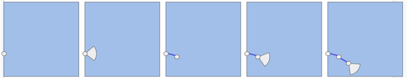
I think this approach would have worked for this figure, since there were never multiple contour lines for the same contour value, but it would have been more finicky, especially around the boundaries, and it would not have generalized to other figures.
Marching Squares
I happened upon a talk by Casey Muratori on YouTube, “Papers I have Loved“, a few weeks ago. One of the papers Casey talked about was Marching Cubes, A High Resolution 3D Surface Construction Algorithm. This 1987 paper by W. Lorenson and H. Cline presented a very simply way to generate surfaces (in 3D or 2D) in places of constant value: \(f(x) = c\).
Casey talked about it in the context of rendering metaballs, but when I found myself presented with the contour problem, it was clear that marching cubes (or squares, rather, since its 2d) was relevant here too.
The algorithm is a simple idea elegantly applied.
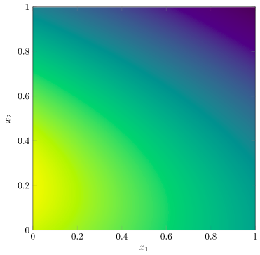
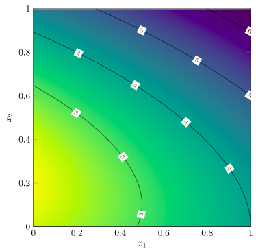
The contour plot we want to make is on a 2d surface in a 3d plot, but let’s just consider the 2d surface for now. Below we show that feasible square along with our objective function, \(f(x) = \|Ax – b\|\):
Our objective is to produce contour lines, the same sort as are produced when we make a PGFPlots contour plot:
We already know that there might be multiple connected contour lines for a given level, so a local search method won’t be sufficient. Instead, marching squares uses a global approach combined with local refinement.
We begin by evaluating a grid of points over our plot:
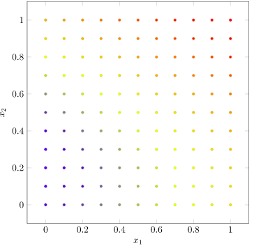
We’ll start with a small grid, but for higher-quality images we’d make it finer.
Let’s focus on the contour line \(f(x) = 3\). We now determine, for each vertex in our mesh, whether its value is above or below our contour target of 3. (I’ll plot the contour line too for good measure):
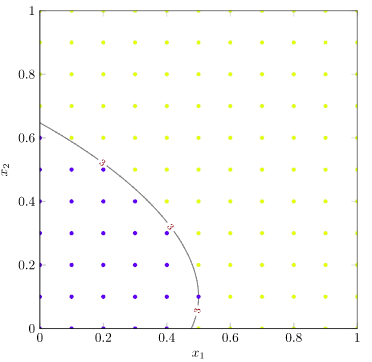
Marching squares will now tile the image based on each 4-vertex square, and the binary values we just evaluated. Any squares with all vertices equal can simply be ignored – the contour line doesn’t pass through them. This leaves the following tiles:
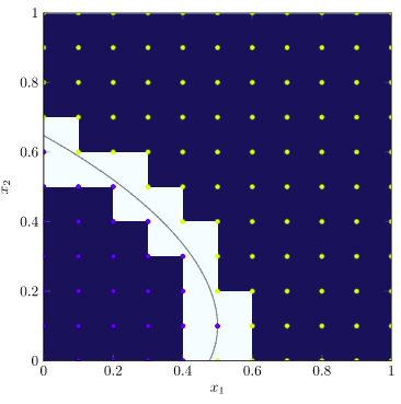
Now, each remaining tile comes in multiple possible “flavors” – the various ways that its vertices can be above or below the objective value. There are \(2^4\) possible tiles, two of which we’ve already discarded, leaving 14 options. The Wikipedia article has a great set of images showing all of the tile combinations, but here we will concern ourselves with two more kinds: tiles with one vertex below or one vertex above, and tiles with two neighboring vertices above and two neighboring vertices below:

Let’s start with the first type. These squares have two edges where the function value changes. We know, since we’re assuming our objective function is continuous, that our contour line must pass through those edges. As such, if we run a bisection search along each of those edges, we can quickly identify those crossing points:
We then get our contour plot, for this particular contour value, by drawing all of the line segments between these crossing points:

We can get higher resolution contour lines by using a finer grid:
To get our full contour plot, we simply run marching squares on multiple contour levels. To get the original plot, I run this algorithm to get all of the little tile line segments, then I render them as separate Linear3 line segments on top of the 3d patch. Pretty cool!
What does the Code Look Like?
The code for marching squares is pretty elegant.
We start off with defining our grid:
nbins = 41
x1s = collect(range(0.0, stop=1.0, length=nbins))
x2s = collect(range(0.0, stop=1.0, length=nbins))
is_above = falses(length(x1s), length(x2s))
Next we define a bisection method for quickly interpolating between two vertices:
function bisect(
    u_target::Float64, x1_lo::Float64, x1_hi::Float64,
    x2_lo::Float64, x2_hi::Float64, k_max::Int=8)
    f_lo = norm(A*[x1_lo, x2_lo, x2_lo]-b)
    f_hi = norm(A*[x1_hi, x2_hi, x2_hi]-b)

    if f_lo > f_hi # need to swap low and high
        x1_lo, x1_hi, x2_lo, x2_hi = x1_hi, x1_lo, x2_hi, x2_lo
    end

    x1_mid = (x1_hi + x1_lo)/2
    x2_mid = (x2_hi + x2_lo)/2
    for k in 1 : k_max
        f_mid = norm(A*[x1_mid, x2_mid, x2_mid] - b)
        if f_mid > u_target
            x1_hi, x2_hi, f_hi = x1_mid, x2_mid, f_mid
        else
            x1_lo, x2_lo, f_lo = x1_mid, x2_mid, f_mid
        end
        x1_mid = (x1_hi + x1_lo)/2
        x2_mid = (x2_hi + x2_lo)/2
    end

    return (x1_mid, x2_mid)
end
In this case I’ve baked in the objective function, but you could of course generalize this and pass one in.
We then iterate over our contour levels. For each contour level (u_target), we evaluate the grid and then evaluate all of our square patches and add little segment plots as necessary:
for (i,x1) in enumerate(x1s)
    for (j,x2) in enumerate(x2s)
        is_above[i,j] = norm(A*[x1, x2, x2] - b) > u_target
    end
end
for i in 2:length(x1s)
    for j in 2:length(x2s)
        # bottom-right, bottom-left, top-right, top-left
        bitmask = 0x00
        bitmask |= (is_above[i,j-1] << 3)
        bitmask |= (is_above[i-1,j-1] << 2)
        bitmask |= (is_above[i,j] << 1)
        bitmask |= (is_above[i-1,j])
        plot = true
        x1_lo1 = x1_hi1 = x2_lo1 = x2_hi1 = 0.0
        x1_lo2 = x1_hi2 = x2_lo2 = x2_hi2 = 0.0
        if bitmask == 0b1100 || bitmask == 0b0011
            # horizontal cut
            x1_lo1, x1_hi1, x2_lo1, x2_hi1 = x1s[i-1], x1s[i-1], x2s[j-1], x2s[j]
            x1_lo2, x1_hi2, x2_lo2, x2_hi2 = x1s[i], x1s[i], x2s[j-1], x2s[j]
        elseif bitmask == 0b0101 || bitmask == 0b1010
            # vertical cut
            x1_lo1, x1_hi1, x2_lo1, x2_hi1 = x1s[i-1], x1s[i], x2s[j-1], x2s[j-1]
            x1_lo2, x1_hi2, x2_lo2, x2_hi2 = x1s[i-1], x1s[i], x2s[j], x2s[j]
        elseif bitmask == 0b1000 || bitmask == 0b0111
            # cut across bottom-right
            x1_lo1, x1_hi1, x2_lo1, x2_hi1 = x1s[i-1], x1s[i], x2s[j-1], x2s[j-1]
            x1_lo2, x1_hi2, x2_lo2, x2_hi2 = x1s[i], x1s[i], x2s[j-1], x2s[j]
        elseif bitmask == 0b0100 || bitmask == 0b1011
            # cut across bottom-left
            x1_lo1, x1_hi1, x2_lo1, x2_hi1 = x1s[i-1], x1s[i], x2s[j-1], x2s[j-1]
            x1_lo2, x1_hi2, x2_lo2, x2_hi2 = x1s[i-1], x1s[i-1], x2s[j-1], x2s[j]
        elseif bitmask == 0b0010 || bitmask == 0b1101
            # cut across top-right
            x1_lo1, x1_hi1, x2_lo1, x2_hi1 = x1s[i-1], x1s[i], x2s[j], x2s[j]
            x1_lo2, x1_hi2, x2_lo2, x2_hi2 = x1s[i], x1s[i], x2s[j-1], x2s[j]
        elseif bitmask == 0b0001 || bitmask == 0b1110
            # cut across top-left
            x1_lo1, x1_hi1, x2_lo1, x2_hi1 = x1s[i-1], x1s[i], x2s[j], x2s[j]
            x1_lo2, x1_hi2, x2_lo2, x2_hi2 = x1s[i-1], x1s[i-1], x2s[j-1], x2s[j]
        else
            plot = false
        end
        if plot
            x1a, x2a = bisect(u_target, x1_lo1, x1_hi1, x2_lo1, x2_hi1)
            x1b, x2b = bisect(u_target, x1_lo2, x1_hi2, x2_lo2, x2_hi2)
            push!(contour_segments,
                Plots.Linear3([x1a, x1b], [x2a, x2b], [x2a, x2b],
                               style="solid, pastelBlue, mark=none")
            )
        end
    end
end
In this code, all we ever do is figure out which two line segments to bisect over, and if we get then, run the bisection and plot the ensuing line. Its actually quite neat and compact.
Conclusion
So there you have it – a home-rolled implementation for contour plotting turns out to be useful for embedding 2d contours in a 3d plot.
Note that the implementation here wasn’t . In this case, we didn’t handle some tile types, namely those where opposing corners have the same aboveness, but neighboring corners have differing aboveness. In those cases, we need to bisect across all four segments, and we typically need to remove ambiguity by sampling in the tile’s center to determine which way the segments cross.
I find it really satisfying to get to apply little bits of knowledge like this from time to time. Its part of computer programming that is endlessly rewarding. I have often been amazed by how a technique that I learned about in one context surprised me by being relevant in something else later on.