In the previous post, we used an LQR controller to solve the classic cart-pole problem. There, the action space is continuous, and our controller is allowed to output any force. This leads to some very smooth control.

We can plot the force over time:
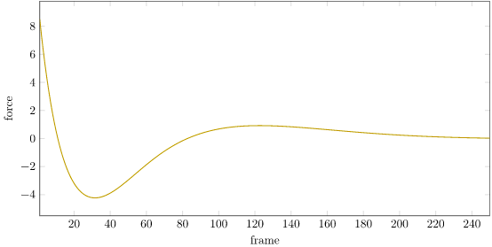
We can see that our force starts off at 8 N and oscillates down to about -4 N before settling down as the cart-pole system stabilizes. This raises a question – don’t real world actuators saturate? What happens if we model that saturation?
LQR with Saturation
The original LQR problem finds the sequence of \(N\) actions (here, cart lateral forces) \(a^{(1)}, \ldots, a^{(N)}\) that produces the sequence of states \(s^{(1)}, \ldots, s^{(N+1)}\) that maximizes the discounted reward across states and actions:
\[\begin{matrix}\underset{\boldsymbol{x}}{\text{maximize}} & R(s^{(1)}, a^{(1)}) + R(s^{(2)}, a^{(2)}) + \ldots + R(s^{(N)}, a^{(N)}) + R_\text{final}(s^{(N+1)}) \\ \text{subject to} & s^{(i+1)} = T_s s^{(i)} + T_a a^{(i)} \qquad \text{ for } i = 1:N \end{matrix}\]
Well, actually we discount future rewards by some factor \(\gamma \in (0,1)\) and we don’t bother with the terminal reward \(R_\text{final}\):
\[\begin{matrix}\underset{\boldsymbol{x}}{\text{maximize}} & R(s^{(1)}, a^{(1)}) + \gamma R(s^{(2)}, a^{(2)}) + \ldots + \gamma^{N-1} R(s^{(N)}, a^{(N)}) \\ \text{subject to} & s^{(i+1)} = T_s s^{(i)} + T_a a^{(i)} \qquad \text{ for } i = 1:N \end{matrix}\]
Or more simply:
\[\begin{matrix}\underset{\boldsymbol{x}}{\text{maximize}} & \sum_{i=1}^N \gamma^{i-1} R(s^{(i)}, a^{(i)}) & \\ \text{subject to} & s^{(i+1)} = T_s s^{(i)} + T_a a^{(i)} & \text{for } i = 1:N \end{matrix}\]
Our dynamics are linear (as seen in the constraint) and our reward is quadratic:
\[R(s, a) = s^\top R_s s + a^\top R_a a\]
It turns out that efficient methods exist for solving this problem exactly (See section 7.8 of Alg4DM), and the solution does not depend on the initial state \(s^{(1)}\).
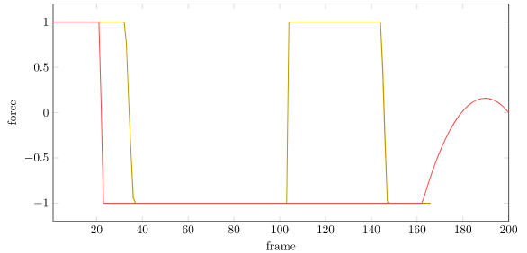
With actuator limits comes force saturation. Now, we could just use the controller that we got without considering saturation, and just clamp its output to a feasible range:

As we can see, our force saturates from the beginning, and is insufficient to stabilize the robot:
We can instead include the saturation constraint in our optimization problem:
\[\begin{matrix}\underset{\boldsymbol{x}}{\text{maximize}} & \sum_{i=1}^N \gamma^{i-1} R(s^{(i)}, a^{(i)}) & \\ \text{subject to} & s^{(i+1)} = T_s s^{(i)} + T_a a^{(i)} & \text{for } i = 1:N \\ & a_\text{min} \leq a^{(i)} \leq a_\text{max} & \text{for } i = 1:N \end{matrix}\]
This problem is significantly more difficult to solve. The added constraints make our problem non-linear, which messes up our previous analysis. Plus, our optimal policy now depends on the initial state.
The problem is still convex though, so we can just throw it into a convex solver and get a solution.
N = 200
a = Convex.Variable(N)
s = Convex.Variable(4, N+1)
problem = maximize(sum(γ^(i-1)*(quadform(s[:,i], Rs) + quadform(a[i], Ra)) for i in 1:N))
problem.constraints += s[:,1] == s₁
for i in 1:N
    problem.constraints += s[:,i+1] == Ts*s[:,i] + Ta*a[i]
    problem.constraints += a_min <= a[i]
    problem.constraints += a[i] <= a_max
end
optimizer = ECOS.Optimizer()
solve!(problem, optimizer)
Solving to 200 steps from the same initial state gives us:

Unfortunately, the gif above shows the optimized trajectory. That’s different than the actual trajectory we get when we use the nonlinear dynamics. There, Little Tippy tips over:
What we really should be doing is re-solve our policy at every time step. Implementing this on a real robot requires getting it to run faster than 50Hz, which shouldn’t be a problem.
Unfortunately, if we implement that, we can’t quite stabilize:

As it turns out, there are states from which Little Tippy, with limited actuation power, does not stabilize with an LQR policy. We can plot the states in which the original LQR policy with infinite actuation stabilizes from \(x = v = 0\) (and does not exceed the \(x\) bounds):
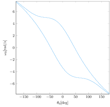
We can produce the same plot for the same LQR policy run with limited actuation:
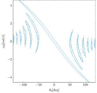
We can see how severe the actuator limits are! To get our robot to really work, we’re going to want to be able to operate despite these actuator limitations. We’re not going to want to assume that we start from somewhere feasible – we’ll want Little Tipple to know how to build up the momentum necessary to swing up the pole and stabilize.
A Cart Pole Search Problem
There are multiple ways that we can get Little Tippy to swing up. We could try something like iLQR, but that won’t necessarily save us from the nonlinear troughs that are the cart-pole problem. It follows a descent direction just like LQR, so unless our problem is convex or we get lucky, we’ll end up in a mere local minimum.
To help Little Tippy find his way to equilibrium, we’ll do something more basic – transform the problem into a search problem. Up until this point, we’ve been using continuous controls techniques to find optimal control sequences. These are excellent for local refinement. Instead, we need to branch out and consider multiple options, and choose between them for the best path to our goal.
We only need a few things to define a search problem:
- A state space \(\mathcal{S}\), which defines the possible system configurations
- An action space \(\mathcal{A}\), which defines the actions available to us
- A deterministic transition function \(T(s,a)\) that applies an action to a state and produces a successor state
- A reward function \(R(s,a)\) that judges a state and the taken action for goodness (higher values are better)
Many search problems additionally define some sort of is_done method that checks whether we are in a terminal (ex: goal) state. For example, in the cart-pole problem, we terminate if Little Tippy deviates too far left or right. We could technically incorporate is_done into our reward, by assigning zero reward whenever we match its conditions, but algorithms like forward search can save some compute by explicitly using it.
The cart-pole problem that we have been solving is already a search problem. We have:
- A state space \(\mathcal{S} = \mathbb{R}^4\) that consists of cart-pole states
- An action space \(\mathcal{A} = \{ a \in \mathbb{R}^1 | a \in [-1,1]\}\) of bounded, continuous force values
- A transition function \(T(s,a)\) that takes a cart-pole state and propagates it with the instantaneous state derivative for \(\Delta t\) to obtain the successor state \(s’\)
- A reward function that, so far, we’ve defined as quadratic in order to apply the LQR machinery, \(R(s,a) = s^\top R_s s + a^\top R_a a\)
Unfortunately, this search problem is made difficult by the fact that it both has an infinite number of actions (since our actions are continuous) and has very long trajectories, as \(\Delta t = 0.02\). Searching for good paths would be pretty difficult. So, what I am going to try is to create a simpler search problem that acts as a higher-level, coarser problem representation, but is powerful enough to let us find our way to our destination.
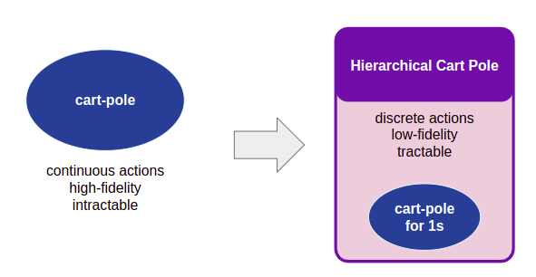
Let’s create a new problem. We’ll call it Hierarchical Cart Pole. The states in this problem are cart-pole states, but the actions are to apply an LQR controller for 1 second. We will create a number of LQR controllers, each for the cart-pole problem linearized around different control points. This gives us the nice smooth control capabilities of an LQR controller, but in
We have:
- A state space \(\mathcal{S} = \mathbb{R}^4\) that consists of cart-pole states
- An action space \(\mathcal{A} = \left\{a_1, a_2, \ldots, a_K \right\}\) that consists of choosing between \(K\) controllers
- A transition function \(T(s,a)\) that takes a cart-pole state and propagates it using the selected LQR controller for 1s
- A reward function:
\[R(s,a) = \begin{cases} \frac{1}{100}r_x + r_\theta & \text{if } x \in [-x_\text{min}, x_\text{max}] \\ 0 & \text{otherwise}\end{cases}\]
The reward function simply gives zero reward for out-of-bounds carts, and otherwise produces more reward the closer Little Tipple is to our target state (\(x = 0, \theta = 0\)). I used \(x_\text{max} = -x_\text{min} = 4.8\) just like the original formulation, \(r_x = x_\text{max}^2 – x^2\), and \(r_\theta = 1 + \cos \theta\).
We can now apply any search algorithm to our Hierarchical Cart Pole problem. I used a simple forward search that tries all possible 4-step action sequences. That is enough to give us pretty nice results:
Starting from rest, Little Tippy builds up momentum and swings up the pole!
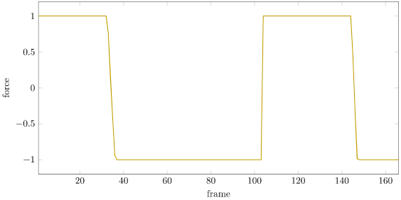
We can plot the forces:
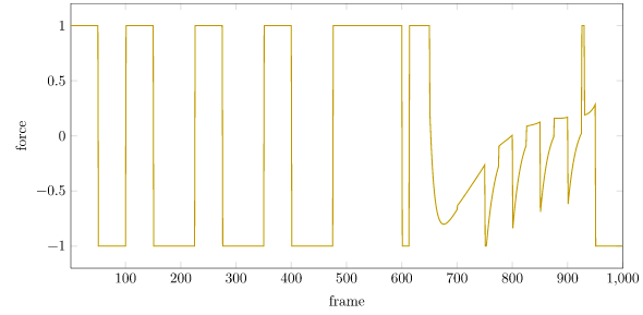
The forces are nice and bounded. We can see the quintessential riding of the rails, with the force bouncing back and forth between its limits. This is quite natural. If we have limits, we’re often going to use everything available to us to get the job done.
In this problem, I linearized the dynamics around 12 control states, all with \(v = \omega = 0\):
reference_states = [
    CartPoleState(-1.0, 0.0, 0.0, 0.0),
    CartPoleState( 0.0, 0.0, 0.0, 0.0),
    CartPoleState( 1.0, 0.0, 0.0, 0.0),
    CartPoleState(-1.0, 0.0, deg2rad(-90), 0.0),
    CartPoleState( 0.0, 0.0, deg2rad(-90), 0.0),
    CartPoleState( 1.0, 0.0, deg2rad(-90), 0.0),
    CartPoleState(-1.0, 0.0, deg2rad(90), 0.0),
    CartPoleState( 0.0, 0.0, deg2rad(90), 0.0),
    CartPoleState( 1.0, 0.0, deg2rad(90), 0.0),
    CartPoleState(-1.0, 0.0, deg2rad(180), 0.0),
    CartPoleState( 0.0, 0.0, deg2rad(180), 0.0),
    CartPoleState( 1.0, 0.0, deg2rad(180), 0.0),
]
We can plot the macro actions as well, which at each time step is the index of the selected reference state:
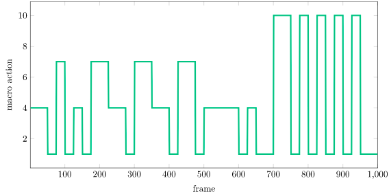
Notice how, at the end, the system chooses 1, which is the LQR controller linearized about \(x = -1\). This is what gets the cart to drive left while remaining stabilized.
Linearization
Alright, I know what you’re thinking. Sweet little solver, but how did you get those LQR controllers?
Before we merely linearized about zero. Now we’re linearizing about other control points.
To do this, we start by linearizing our equations of motion. This means we’re forming the 1st order Taylor approximation. The first-order Taylor approximation of some function \(g(x)\) about a reference \(x_\text{ref}\) is \(g(x) \approx g(x_\text{ref}) + g'(x_\text{ref}) (x – x_\text{ref})\). If the equations of motion are \( \dot{s} = F(s, a)\), then the 1st order Taylor approximation about a reference state \(s_\text{ref}\) and a reference action \(a_\text{ref}\) is
\[\dot{s} \approx F(s_\text{ref}, a_\text{ref}) + J_s \cdot (s – s_\text{ref}) + J_a \cdot (a – a_\text{ref})\]
where \(J_s\) and \(J_a\) are the state and action Jacobians (matrices of gradients). Here I always used a reference action of zero.
Why compute this by hand when you could have the computer do it for you? This is what auto-differentiating packages like Zygote.jl are for. I ended up using Symbolics.jl so I could see the symbolic output:
function linearize(mdp::CartPole, s_ref::CartPoleState)
    Δt = mdp.Δt
    @variables x v θ ω ℓ g m M F
    η = (F + m*ℓ*sin(θ)*ω^2) / M
    pole_α = simplify((M*g*sin(θ) - M*η*cos(θ))/(ℓ*(4//3*M - m*cos(θ)^2)))
    cart_a = simplify(η - m * ℓ * pole_α * cos(θ) / M)
    # Our first order derivatives
    equations_of_motion = [
        v,
        cart_a,
        ω,
        pole_α
    ]
    state_vars = [x,v,θ,ω]
    action_vars = [F]
    ns = length(state_vars)
    na = length(action_vars)
    df = Array{Float64}(undef, ns)
    Js = Array{Float64}(undef, ns, ns)
    Ja = Array{Float64}(undef, ns, na)
    subs = Dict(x => s_ref.x, v => s_ref.v, θ => s_ref.θ, ω => s_ref.ω,
                m => mdp.mass_pole, M => mdp.mass_pole + mdp.mass_cart,
                g => mdp.gravity, ℓ => mdp.pole_length, F => 0.0)
    for (i, eom) in enumerate(equations_of_motion)
        df[i] = value.(substitute.(eom, (subs,))[1])
        for (j, var) in enumerate(state_vars)
            derivative = expand_derivatives(Differential(var)(eom))
            Js[i,j] = value.(substitute.(derivative, (subs,))[1])
        end
        for (j, var) in enumerate(action_vars)
            derivative = expand_derivatives(Differential(var)(eom))
            Ja[i,j] = value.(substitute.(derivative, (subs,))[1])
        end
    end
    return (df, Js, Ja)
end
The intermediate system, before the reference state is substituted in, is:
\[\begin{bmatrix} \dot{x} \\ \dot{v} \\ \dot{\theta} \\ \dot{\omega} \end{bmatrix} \approx \left. \begin{bmatrix} v \\ \zeta – \frac{m_p \ell \ddot{\theta} \cos(\theta)}{m_p + m_c} \\ \omega \\ \frac{g\sin(\theta) – \zeta \cos(\theta)}{\ell\left( \frac{4}{3} – \frac{m_p \cos(\theta)^2}{m_p + m_c} \right)} \end{bmatrix} \right|_{s = s_\text{ref}} + \left. \begin{bmatrix} 0 & 1 & 0 & 0 \\ 0 & 0 & \frac{-m_p g}{\frac{4}{3}M – m_p} & \frac{\partial}{\partial \omega} \ddot{x} \\ 0 & 0 & 0 & 1 \\ 0 & 0 & \frac{Mg}{\ell \left(\frac{4}{3}M – m_p\right)} & \frac{-m_p \omega \sin (2 \theta)}{\frac{4}{3}M – m_p \cos^2 (\theta)} \end{bmatrix}\right|_{s = s_\text{ref}} \begin{bmatrix} x \\ v \\ \theta \\ \omega \end{bmatrix} + \left. \begin{bmatrix} 0 \\ \frac{\frac{4}{3}}{\frac{4}{3}M – m_p} \\ 0 \\ -\frac{1}{\ell\left(\frac{4}{3}M – m_p\right)}\end{bmatrix}\right|_{s = s_\text{ref}} a\]
where \(\ell\) is the length of the pole, \(m_p\) is the mass of the pole, \(M = m_p + m_c\) is the total mass of the cart-pole system,
\[\zeta = \frac{a + m_p \ell \sin(\theta) \omega^2}{m_p + m_c}\text{,}\]
and
\[\frac{\partial}{\partial \omega} \ddot{x} = m_p \omega \ell \frac{m_p \cos (\theta)\sin(2\theta) – 2 m_p\cos^2(\theta) \sin (\theta) + \frac{8}{3}M \sin(\theta)}{M\left(\frac{4}{3}M – m_p\cos^2(\theta)\right)}\]
For example, linearizing around \(s_\text{ref} = [1.0, 0.3, 0.5, 0.7]\) gives us:
\[\begin{bmatrix} \dot{x} \\ \dot{v} \\ \dot{\theta} \\ \dot{\omega} \end{bmatrix} \approx \begin{bmatrix} \hphantom{-}0.300 \\ -0.274 \\ \hphantom{-}0.700 \\ \hphantom{-}3.704 \end{bmatrix} + \begin{bmatrix} 0 & 1 & 0 & 0 \\ 0 & 0 & -0.323 & 0.064 \\ 0 & 0 & 0 & 1 \\ 0 & 0 & 6.564 & -0.042 \end{bmatrix} \begin{bmatrix} x \\ v \\ \theta \\ \omega \end{bmatrix} + \begin{bmatrix} 0 \\ \hphantom{-}0.959 \\ 0 \\ -0.632\end{bmatrix} a\]
We’re not quite done yet. We want to get our equations into the form of linear dynamics, \(s’ = T_s s + T_a a\). Just as before, we apply Euler integration to our linearized equations of motion:
\[\begin{aligned}s’ & \approx s + \Delta t \dot{s} \\ &= s + \Delta t \left( F(s_\text{ref}, a_\text{ref}) + J_s \cdot (s – s_\text{ref}) + J_a a \right) \\ &= s + \Delta t F(s_\text{ref}, a_\text{ref}) + \Delta t J_s s – \Delta t J_s s_\text{ref} + \Delta t J_a a \\ &= \left(I + \Delta t J_s \right) s + \left( \Delta t F(s_\text{ref}, a_\text{ref}) – \Delta t J_s s_\text{ref} \right) + \Delta t J_a a \end{aligned}\]
So, to get it in the form we want, we have to introduce a 5th state that is always 1. This gives us the linear dynamics we want:
\[\begin{bmatrix} s \\ 1 \end{bmatrix} \approx \begin{bmatrix} I + \Delta t J_s & \Delta t F(s_\text{ref}, a_\text{ref}) – \Delta t J_s s_\text{ref} \\ [0\>0\>0\>0] & 1 \end{bmatrix} \begin{bmatrix} s \\ 1\end{bmatrix} + \begin{bmatrix} \Delta t J_a \\ 0 \end{bmatrix} a\]
For the example reference state above, we get:
\[\begin{bmatrix}x’ \\ v’ \\ \theta’ \\ \omega’ \\ 1\end{bmatrix} \approx \begin{bmatrix}1 & 0.02 & 0 & 0 & 0 \\ 0 & 1 & -0.00646 & 0.00129 & -0.00315 \\ 0 & 0 & 1 & 0.02 & 0 \\ 0 & 0 & 0.131 & 0.999 & 0.00903 \\ 0 & 0 & 0 & 0 & 1\end{bmatrix}\begin{bmatrix}x \\ v \\ \theta \\ \omega \\ 1\end{bmatrix} + \begin{bmatrix}0 \\ 0.019 \\ 0 \\ -0.0126 \\ 0\end{bmatrix}\]
We can take our new \(T_s\) and \(T_a\), slap an extra dimension onto our previous \(R_s\), and use the same LQR machinery as in the previous post to come up with a controller. This gives us a new control \(K\), which we use as a policy:
\[\pi(s) = K \begin{bmatrix}x – x_\text{ref} \\ v – v_\text{ref} \\ \text{angle_dist}(\theta, \theta_\text{ref}) \\ \omega – \omega_\text{ref} \\ 1\end{bmatrix}\]
For our running example, \(K = [2.080, 3.971, 44.59, 17.50, 2.589]\). Notice how the extra dimension formulation can give us a constant force component.
The policy above was derived with the \(R_s\) from the previous post, diagm([-5, -1, -5, -1]). As an aside, we can play around with it to get some other neat control strategies. For example, we can set the first element to zero if we want to ignore \(x\) and control about velocity. Below is a controller that tries to balance the pole while maintaining \(v = 1\):
That is how you might develop a controller for, say, an RC car that you want to stay stable around an input forward speed.
Conclusion
In this post we helped out Little Tippy further by coming up with a control strategy by which he could get to stability despite having actuator limits. We showed that it could (partially) be done by explicitly incorporating the limits into the linearized optimization problem, but that this was limited to the small local domain around the control point. For larger deviations we used a higher-level policy that selected between multiple LQR strategies to search for the most promising path to stability.
I want to stress that the forward search strategy used isn’t world-class by any stretch of the imagination. It does, however, exemplify the concept of tackling a high-resolution problem that we want to solve over an incredibly long time horizon (cart-pole swingup) with a hierarchical approach. We use LQR theory for what it does best – optimal control around a reference point – and build a coarser problem around it that uses said controllers to achieve our goals.