In the previous two posts, we used various control strategies to solve the classic cart-pole problem. In the first, we used a classic LQR controller to stabilize the cart pole in the vicinity of its equilibrium point. In the second, we built a system that could reach stability from anywhere, by forming a hierarchical problem using LQR controllers around various reference states and a top-level search strategy to find the right sequence of controls to reach stability.

All of this was well and good, but what if we change our problem even more drastically?

So far, everything we have worked with has had intimate knowledge of the underlying dynamics. The LQR approach only works because we know the equations of motion, and can take the necessary derivatives to form a linear system. What if we didn’t have those equations of motion? In many real-world cases, we simply don’t. Now we’re going to pretended we don’t know the equations of motion, and will learn a good controller anyways.

From Controls to Reinforcement Learning

We are going to take a journey, leaving the land of controls behind, and head to the realm of reinforcement learning. This land is at first glance completely foreign, but once you get your bearings you begin to realize their strange customs are really just alternate manifestations of things we’re already used to.

Previously, in the land of controls, we derived controllers that produced control inputs to drive the system’s state to equilibrium while minimizing cost. The people of the realm of reinforcement learning do the same thing, except they find policies \(\pi(s)\) that produce actions to drive the system’s state to equilibrium while maximizing reward.

Now, unlike in the land of controls, the people of the realm of reinforcement learning are very used to working on systems where they do not know the equations of motion. They know that a transition function \(T(s’\mid s,a)\) and a reward function \(R(s,a)\) exist, but do not necessarily know what it is. Instead, they allow their agent to interact with its environment, and thereby gain information about these from the state transitions and rewards observed.

In this post I am going to use an actor-critic method. These are covered in chapter 13 of Alg4DM. The “actor” part refers to the fact that we learn a policy that our agent then follows. The “critic” part refers to the fact that we also learn a value function that critiques the agent’s policy. Both are trained in parallel, the critic becoming better at maximizing the critic’s reward, and the critic getting better at reflecting the true value of the actor’s behavior.

Problem Definition

We always start by defining the actual problem we are solving. This is super important. The problem that we solve is always a model of the ground truth. As George Box famously said, “All models are wrong, some models are useful.” The real world doesn’t care that modeling actuator saturation is harder – it will simply do what it always does.

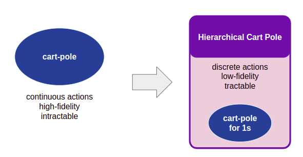
To shake things up a tad, we are going to use cart pole with discrete actions, as it was originally presented. Note that in the land of controls we worked with continuous actions. (We could totally do that here – its just nice to do something different).

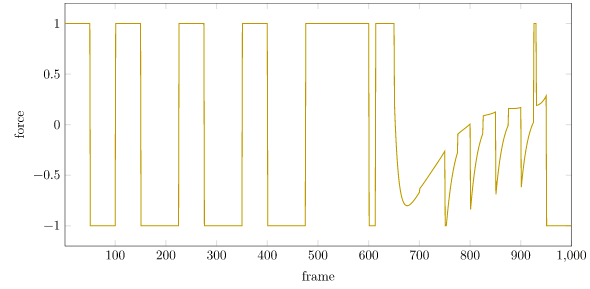
Now, the real robot likely can exert continuous forces. We are making a modeling choice, and have to live with the consequences. A series of discrete force outputs will naturally be more jerky / stuttery than a nice smooth output. Maybe we’ll want to tidy that up later, perhaps with a low-pass filter. For now, we’ll go with this.

As such, our problem definition is:

• State Space \(\mathcal{S}\): The same classic cart-pole states consisting of the lateral position \(x\), the lateral velocity \(v\), the pole angle \(\theta\), and the pole’s angular rate \(\omega\).
• Action Space \(\mathcal{A}\): We assume the cart has a maximum actuation force of \(F\). The available actions at each time step (same time step of 50Hz as before) are \(F\), \(0\), and \(-F\). As such, we have three discrete actions.
• Transition Function \(T(s’\mid s, a)\): We use the deterministic cart-pole transition function under the hood, with the same transition dynamics that we have already been using.
• Reward Function \(R(s,a)\): The original paper just gives a reward of 1 any time the cart is in-bounds in \(x\) and \(\theta\). We are instead going to use the reward function formulation that penalizes deviations from stability:
  \[R(s,a) = \frac{1}{100}r_x + r_\theta = \frac{1}{100}(\Delta x_\text{max}^2 – x^2) + (1 + \cos(\theta))\]
  We continue to give zero reward if we are out of bounds in \(x\), but not in \(\theta\).

Note that our learning system does not know the details of the transition and reward function. Note also that our reward function is non-negative, which isn’t necessary, but can make things a bit more intuitive.

Vanilla Actor Critic

The core ideas of actor-critic are pretty straightforward. We are simultaneously learning a policy and a value function.

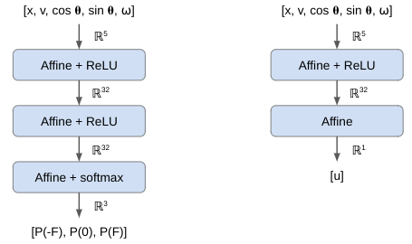
Our policy, (which is stochastic to make the math easier), is a function that produces a categorical distribution over our three actions. We’re going to use a simply deep neural net for this, one with three fully connected layers:

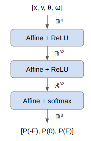
Notice the softmax activation function on the final layer, which ensures that our output is a valid probability distribution.

There are multiple actor-critic approaches with different value functions. In this case I’ll learn a state-value function \(U(s)\), which predicts the expected reward from the given state (the discounted sum of all future rewards). I’m also going to use a simple neural network for this:

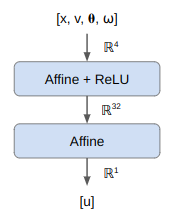
The final layer has no activation function, so the out put can be any real number.

These can both readily be defined using Flux.jl:

get_stochastic_policy(n_hidden::Int=32) = Chain(Dense(4 => n_hidden,relu), Dense(n_hidden => n_hidden,relu), Dense(n_hidden => 3), softmax)
get_value_function(n_hidden::Int=32) = Chain(Dense(4 => n_hidden,relu), Dense(n_hidden => 1))

In every iteration we run a bunch of rollouts and:

• compute a policy gradient to get it to maximize the value functions
• compute a value gradient to get our value function to reflect the true expected value

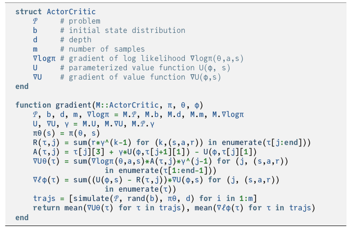
Alg4DM presents this in one nicely compact pseudocode block:

This formulation uses the likelihood ration approach to computing the policy gradient, which for a stochastic policy is:

\[\nabla U(\theta) = \underset{\tau}{\mathbb{E}}\left[\sum_{k=1}^d \gamma^{k-1} \nabla_\theta \log \pi_\theta\left(a^{(k)}\mid s^{(k)}\right) A_\theta\left(s^{(k)},a^{(k)}\right)\right]\]

where we estimate the advantage using our critic value function:

\[A_\theta(s,a) = \underset{r, s’}{\mathbb{E}}\left[ r + \gamma U_\phi(s’) – U_\phi(s)\right]\]

For the critic, we simply minimize the difference between the predicted expected value \(U_\phi(s)\) and the expected value obtained by running the current policy \(U^{\pi_\theta}(s)\):

\[\ell(\phi) = \frac{1}{2}\underset{s}{\mathbb{E}}\left[\left(U_\phi(s) – U^{\pi_\theta}(s)\right)^2\right]\]

The critic gradient is thus:

\[\nabla \ell(\phi) = \underset{s}{\mathbb{E}}\left[ \sum_{k=1}^d \left( U_\phi(s^{(k)}) – r_\text{to-go}^{(k)} \right) \nabla_\phi U_\phi(s^{(k)}) \right]\]

While the math may look a bit tricky, the code block above shows how straightforward it is to implement. You just simulate a bunch of rollouts (\(\tau\)), and then calculate the gradients.

The code I wrote is functionally identical to the code in the textbook, but is laid out a bit differently to help with legibility (and later expansion). Notice that I compute a few extra things so we can plot them later:

function run_epoch(
    M::ActorCritic,
    π::Chain, # policy π(s)
    U::Chain,  # value function U(s)
    mem::ActorCriticMemory,
    )
    t_start = time()
    𝒫, d_max, m = M.𝒫, M.d, M.m
    data = ActorCriticData()
    params_π, params_U = Flux.params(π), Flux.params(U)
    ∇π, ∇U, vs, Us = mem.∇π, mem.∇U, mem.vs, mem.Us
    states, actions rewards = mem.states, mem.actions, mem.rewards
    a_selected = [0.0,0.0,0.0]
    # Zero out the gradients
    for grad in ∇π
        fill!(grad, 0.0)
    end
    for grad in ∇U
        fill!(grad, 0.0)
    end
    # Run m rollouts and accumulate the gradients.
    for i in 1:m
        # Run a rollout, storing the states, actions, and rewards.
        # Keep track of max depth reached.
        max_depth_reached = rollout(M, π, U, mem)
        fit!(data.max_depth_reached, max_depth_reached)
        # Compute the actor and critic gradients
        r_togo = 0.0
        for d in max_depth_reached:-1:1
            v = vs[d]
            s = states[d]
            a = actions[d]
            r = rewards[d]
            s′ = states[d+1]
            a_selected[1] = 0.0
            a_selected[2] = 0.0
            a_selected[3] = 0.0
            a_selected[a] = 1.0
            r_togo = r + γ*r_togo
            A = r_togo - Us[d]
            fit!(data.advantage, A)
            ∇logπ = gradient(() -> A*γ^(d-1)*log(π(v) ⋅ a_selected), params_π)
            ∇U_huber = gradient(() -> Flux.Losses.huber_loss(U(v), r_togo), params_U)
            for (i_param,param) in enumerate(params_π)
                ∇π[i_param] -= ∇logπ[param]
            end
            for (i_param,param) in enumerate(params_U)
                ∇U[i_param] += ∇U_huber[param]
            end
        end
    end
    # Divide to get the mean
    for grad in ∇π
        grad ./= m
    end
    for grad in ∇U
        grad ./= m
    end
    data.∇_norm_π = sqrt(sum(sum(v^2 for v in grad) for grad in ∇π))
    data.∇_norm_U = sqrt(sum(sum(v^2 for v in grad) for grad in ∇U))
    data.w_norm_π = sqrt(sum(sum(w^2 for w in param) for param in params_π))
    data.w_norm_U = sqrt(sum(sum(w^2 for w in param) for param in params_U))
    data.t_elapsed = time() - t_start
    return (∇π, ∇U, data)
end

Theoretically, that is all you need to get things to work. Each iteration you run a bunch of rollouts, accumulate gradients, and then use these gradients to update both the policy and the value function parameterizations. You keep iterating until the parameterizations converge.

With such an implementation, we get the striking result of….

As we can see, the policy isn’t doing too well. What did we do wrong?

Theoretically, nothing wrong, but practically, we’re missing some bells and whistles that make a massive difference. These sorts of best practices are incredibly important in reinforcement learning (and generally in deep learning).

Decomposing our Angles

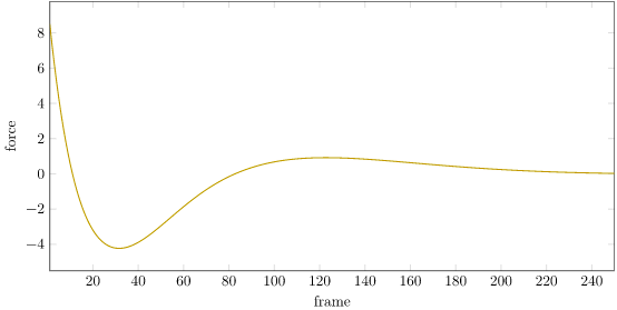
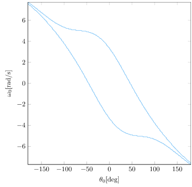
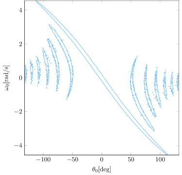
The first change we are going to make is to the inputs to our deep neural net. The current inputs use the raw angle, \(\theta\). This may work well in the basic cart-pole problem where our angle is bounded within a small range, but in a more general cart-pole setting where the pole can rotate multiple times, we end up with weird angular effects that are difficult for a neural network to learn how to handle:

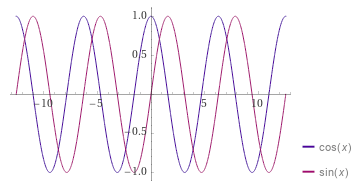
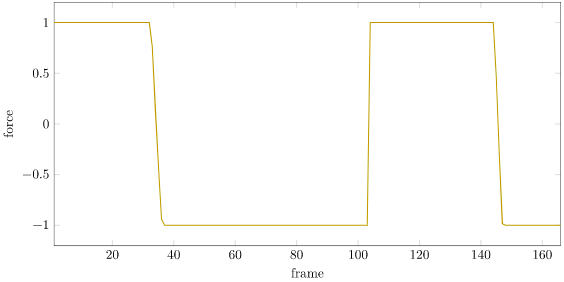
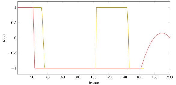
In order to better handle the angle, we are going to instead input \(\cos(\theta)\) and \(\sin(\theta)\):

Wrangling the Loss Functions

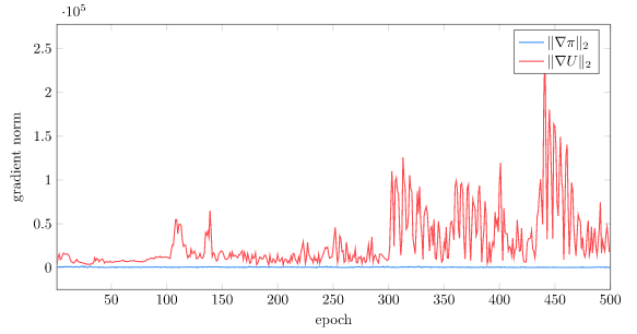
One of the biggest issues we have is with the reward function. The expected value at a given state can be quite large. A single state can \(R(s,a)\) produce values as large as 4.8^2/100 + 2 = 2.23, but these then get accumulated over 2000 time steps with a discount factor of \(\gamma = 0.995\), resulting in values as large as \(U(s) = \sum_{k=1}^2000 2.23 \gamma^{k-1} \approx 446\). Now, 446 isn’t massive, but it is still somewhat large. Pretty much everything deep-learning likes to work close to zero.

We can plot our gradient norm during training to see how this large reward can cause an issue. The magnitude of the value function gradient is massive! This leads to large instabilities, particularly late in training:

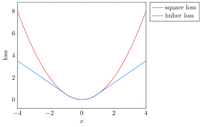
The first thing we will do is dampen out the loss signal for large deviations in reward. Right now, if we predict, say, \(U(s) = 50\) but the real reward is \(U(s) = 400\), we’d end up with a squared loss value of \(350^2 = 122500\). That is somewhat unwieldy.

We want to use a squared loss, for its simplicity and curvature, but only if we are pretty close to the correct value. If we are far off the mark, we’d rather use something gentler.

So we’ll turn to the Huber loss, which uses the squared loss for nearly accurate values and a linear loss for sufficiently inaccurate values:

This helps alleviate the large reward problem, but we can do better. The next thing we will do is normalize our expected values. This step adjusts the expected values to have mean zero and a unit standard deviation (i.e., follow a normal distribution):

\[\bar{u} = (u – \mu) / \sigma\]

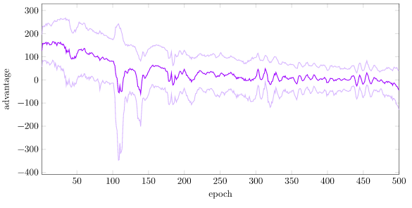
Right now, our average advantage starts off very large (~150), with a large standard deviation (~50), and over time settles to around mean 0 and stdev 30:

To normalize, we need to keep a running estimate of the value function mean \(\mu\) and standard deviation \(\sigma\). OnlineStats.jl makes this easy. One important thing to note, however, is that we compute the reward-to-go for multiple depths, and the estimated values are going to be different depending on the depth. A reward-to-go from \(k=1\) with a max depth of 2000 is going to be different than a reward-to-go from \(k=1999\). As such, we actually maintain separate mean and standard deviation estimates for each depth.

The last thing we do is clamping, both to the standardized reward-to-go:

r_togo = r + γ*r_togo
r_togo_standardized = (r_togo - r_togo_μs[d]) / (r_togo_σs[d] + 1e-3)
r_togo_standardized = clamp(r_togo_standardized, -max_standardized_r_togo, max_standardized_r_togo)
fit!(r_togo_est[d], r_togo)

and to the gradient:

for grad in ∇π
    grad ./= m
    clamp!(grad, -max_gradient, max_gradient)
end
for grad in ∇U
    grad ./= m
    clamp!(grad, -max_gradient, max_gradient)
end

Together, these changes allow the value function to predict values with zero-mean and unit variance, which is a lot easier to learn than widely-ranging large values. This is especially important here because the true value function values depend on the policy, which is changing. A normalized reward will consistently be positive for “good” states and negative for “bad” states, whereas a non-normalized will be some large value for “good” states and some not as large value for “bad” states. Normalization thus stabilizes learning.

Regularization

The final change to include is regularization. I am not certain that this makes a huge difference here, but it often does when working with deep learning projects.

Directly minimizing the critic loss and maximizing the expected policy reward can often be achieved with multiple parameterizations. These parameterizations may be on different scales. As we’ve seen before, we don’t like working with large (in an absolute sense) numeric values. Regularization adds a small penalty for large neural network weights, thereby breaking ties and causing the process to settle on a smaller parameterization.

The math is simple if we try to minimize the squared size our parameters:

\[\ell_\text{regularization}(\theta) = \frac{1}{2} \theta^\top \theta\]

Here, the gradient is super simple:

\[\nabla \ell_\text{regularization}(\theta) = \theta\]

We can thus simply add in our parameter values, scaled by a regularization weight:

for (param, grad) in zip(params_π, ∇π)
    grad += M.w_reg_π * param  # regularization term
    Flux.update!(opt_π, param, grad)
end
for (param, grad) in zip(params_U, ∇U)
    grad += M.w_reg_U * param
    Flux.update!(opt_U, param, grad)
end

Putting it all Together

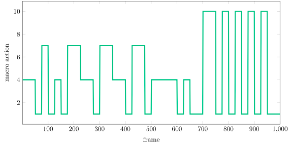
With all of these changes in place, learning is much better. We are able to get Little Tippy the robot to stabilize:

The performance isn’t perfect, because we are, after all, working without explicit knowledge of the system dynamics, and are outputting discrete forces. Nevertheless, this approach was able to figure it out.

The policy was trained for 500 epochs, each with 128 rollouts to a maximum depth of 1000. A rollout terminates if the cart-pole gets further than 4.8m from the origin. The policy pretty quickly figures out how to stay within bounds: (plus or minus one stdev are also shown):

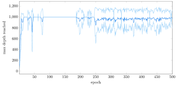
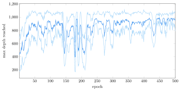
For contrast, here is the same plot with the vanilla setup:

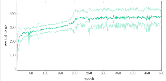
The actual performance is better measured by the mean reward-to-go (i.e., expected value) that the system maintains over time. We can see that we have more-or-less converged:

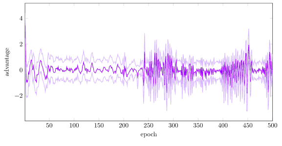
With regularization, our advantage is nicely kept roughly standardized:

Conclusion

Actor-critic methods are nice for many more general problems, because we often do not know real-world dynamics. Neural networks can be very good function approximations, adapting to the problem at hand (whether that be Go, or an aircraft controller). That being said, actor-critic methods alone are not a panacea, and still require special knowledge and insight. In this post alone, we covered the following decision points that we as a designer made:

• Whether to use discrete actions
• The cart-pole reward function
• Which policy gradient method to use
• Which critic loss function to minimize
• Maximum rollout depth
• Number of rollouts per epoch
• Number of epochs / training termination condition
• Policy neural network architecture
• Critic neural network architecture
• Neural network weight initialization method
• Whether to use gradient clamping
• Using sine and cosine rather than raw angles
• Standardizing the expected value (reward-to-go)
• Which optimizer to use (I used Adam).

Being a good engineer often requires being aware of so much more than the vanilla concepts. It is especially important to understand when one is making a decision, and what impact that design has.

Thank you for reading!

The code for this post is available here. A notebook is here.

In the previous post, we used an LQR controller to solve the classic cart-pole problem. There, the action space is continuous, and our controller is allowed to output any force. This leads to some very smooth control.

We can plot the force over time:

We can see that our force starts off at 8 N and oscillates down to about -4 N before settling down as the cart-pole system stabilizes. This raises a question – don’t real world actuators saturate? What happens if we model that saturation?

LQR with Saturation

The original LQR problem finds the sequence of \(N\) actions (here, cart lateral forces) \(a^{(1)}, \ldots, a^{(N)}\) that produces the sequence of states \(s^{(1)}, \ldots, s^{(N+1)}\) that maximizes the discounted reward across states and actions:

\[\begin{matrix}\underset{\boldsymbol{x}}{\text{maximize}} & R(s^{(1)}, a^{(1)}) + R(s^{(2)}, a^{(2)}) + \ldots + R(s^{(N)}, a^{(N)}) + R_\text{final}(s^{(N+1)}) \\ \text{subject to} & s^{(i+1)} = T_s s^{(i)} + T_a a^{(i)} \qquad \text{ for } i = 1:N \end{matrix}\]

Well, actually we discount future rewards by some factor \(\gamma \in (0,1)\) and we don’t bother with the terminal reward \(R_\text{final}\):

\[\begin{matrix}\underset{\boldsymbol{x}}{\text{maximize}} & R(s^{(1)}, a^{(1)}) + \gamma R(s^{(2)}, a^{(2)}) + \ldots + \gamma^{N-1} R(s^{(N)}, a^{(N)}) \\ \text{subject to} & s^{(i+1)} = T_s s^{(i)} + T_a a^{(i)} \qquad \text{ for } i = 1:N \end{matrix}\]

Or more simply:

\[\begin{matrix}\underset{\boldsymbol{x}}{\text{maximize}} & \sum_{i=1}^N \gamma^{i-1} R(s^{(i)}, a^{(i)}) & \\ \text{subject to} & s^{(i+1)} = T_s s^{(i)} + T_a a^{(i)} & \text{for } i = 1:N \end{matrix}\]

Our dynamics are linear (as seen in the constraint) and our reward is quadratic:

\[R(s, a) = s^\top R_s s + a^\top R_a a\]

It turns out that efficient methods exist for solving this problem exactly (See section 7.8 of Alg4DM), and the solution does not depend on the initial state \(s^{(1)}\).

With actuator limits comes force saturation. Now, we could just use the controller that we got without considering saturation, and just clamp its output to a feasible range:

As we can see, our force saturates from the beginning, and is insufficient to stabilize the robot:

We can instead include the saturation constraint in our optimization problem:

\[\begin{matrix}\underset{\boldsymbol{x}}{\text{maximize}} & \sum_{i=1}^N \gamma^{i-1} R(s^{(i)}, a^{(i)}) & \\ \text{subject to} & s^{(i+1)} = T_s s^{(i)} + T_a a^{(i)} & \text{for } i = 1:N \\ & a_\text{min} \leq a^{(i)} \leq a_\text{max} & \text{for } i = 1:N \end{matrix}\]

This problem is significantly more difficult to solve. The added constraints make our problem non-linear, which messes up our previous analysis. Plus, our optimal policy now depends on the initial state.

The problem is still convex though, so we can just throw it into a convex solver and get a solution.

N = 200
a = Convex.Variable(N)
s = Convex.Variable(4, N+1)
problem = maximize(sum(γ^(i-1)*(quadform(s[:,i], Rs) + quadform(a[i], Ra)) for i in 1:N))
problem.constraints += s[:,1] == s₁
for i in 1:N
    problem.constraints += s[:,i+1] == Ts*s[:,i] + Ta*a[i]
    problem.constraints += a_min <= a[i]
    problem.constraints += a[i] <= a_max
end
optimizer = ECOS.Optimizer()
solve!(problem, optimizer)

Solving to 200 steps from the same initial state gives us:

Unfortunately, the gif above shows the optimized trajectory. That’s different than the actual trajectory we get when we use the nonlinear dynamics. There, Little Tippy tips over:

What we really should be doing is re-solve our policy at every time step. Implementing this on a real robot requires getting it to run faster than 50Hz, which shouldn’t be a problem.

Unfortunately, if we implement that, we can’t quite stabilize:

As it turns out, there are states from which Little Tippy, with limited actuation power, does not stabilize with an LQR policy. We can plot the states in which the original LQR policy with infinite actuation stabilizes from \(x = v = 0\) (and does not exceed the \(x\) bounds):

We can produce the same plot for the same LQR policy run with limited actuation:

We can see how severe the actuator limits are! To get our robot to really work, we’re going to want to be able to operate despite these actuator limitations. We’re not going to want to assume that we start from somewhere feasible – we’ll want Little Tipple to know how to build up the momentum necessary to swing up the pole and stabilize.

A Cart Pole Search Problem

There are multiple ways that we can get Little Tippy to swing up. We could try something like iLQR, but that won’t necessarily save us from the nonlinear troughs that are the cart-pole problem. It follows a descent direction just like LQR, so unless our problem is convex or we get lucky, we’ll end up in a mere local minimum.

To help Little Tippy find his way to equilibrium, we’ll do something more basic – transform the problem into a search problem. Up until this point, we’ve been using continuous controls techniques to find optimal control sequences. These are excellent for local refinement. Instead, we need to branch out and consider multiple options, and choose between them for the best path to our goal.

We only need a few things to define a search problem:

• A state space \(\mathcal{S}\), which defines the possible system configurations
• An action space \(\mathcal{A}\), which defines the actions available to us
• A deterministic transition function \(T(s,a)\) that applies an action to a state and produces a successor state
• A reward function \(R(s,a)\) that judges a state and the taken action for goodness (higher values are better)

Many search problems additionally define some sort of is_done method that checks whether we are in a terminal (ex: goal) state. For example, in the cart-pole problem, we terminate if Little Tippy deviates too far left or right. We could technically incorporate is_done into our reward, by assigning zero reward whenever we match its conditions, but algorithms like forward search can save some compute by explicitly using it.

The cart-pole problem that we have been solving is already a search problem. We have:

• A state space \(\mathcal{S} = \mathbb{R}^4\) that consists of cart-pole states
• An action space \(\mathcal{A} = \{ a \in \mathbb{R}^1 | a \in [-1,1]\}\) of bounded, continuous force values
• A transition function \(T(s,a)\) that takes a cart-pole state and propagates it with the instantaneous state derivative for \(\Delta t\) to obtain the successor state \(s’\)
• A reward function that, so far, we’ve defined as quadratic in order to apply the LQR machinery, \(R(s,a) = s^\top R_s s + a^\top R_a a\)

Unfortunately, this search problem is made difficult by the fact that it both has an infinite number of actions (since our actions are continuous) and has very long trajectories, as \(\Delta t = 0.02\). Searching for good paths would be pretty difficult. So, what I am going to try is to create a simpler search problem that acts as a higher-level, coarser problem representation, but is powerful enough to let us find our way to our destination.

Let’s create a new problem. We’ll call it Hierarchical Cart Pole. The states in this problem are cart-pole states, but the actions are to apply an LQR controller for 1 second. We will create a number of LQR controllers, each for the cart-pole problem linearized around different control points. This gives us the nice smooth control capabilities of an LQR controller, but in a search problem that we can actually do things with.I feel like this trick is a big secret of the universe. If a problem is too hard to solve, break it up into a coarser problem that you can solve. We don't fly planes with a single controller, but do hierarchical control. Humans don't reason about every muscle twitch when walking somewhere, but can reason at the level of Google maps and leave lower-level walking actions to muscle memory.

We have:

• A state space \(\mathcal{S} = \mathbb{R}^4\) that consists of cart-pole states
• An action space \(\mathcal{A} = \left\{a_1, a_2, \ldots, a_K \right\}\) that consists of choosing between \(K\) controllers
• A transition function \(T(s,a)\) that takes a cart-pole state and propagates it using the selected LQR controller for 1s
• A reward function:
  \[R(s,a) = \begin{cases} \frac{1}{100}r_x + r_\theta & \text{if } x \in [-x_\text{min}, x_\text{max}] \\ 0 & \text{otherwise}\end{cases}\]

The reward function simply gives zero reward for out-of-bounds carts, and otherwise produces more reward the closer Little Tipple is to our target state (\(x = 0, \theta = 0\)). I used \(x_\text{max} = -x_\text{min} = 4.8\) just like the original formulation, \(r_x = x_\text{max}^2 – x^2\), and \(r_\theta = 1 + \cos \theta\).

We can now apply any search algorithm to our Hierarchical Cart Pole problem. I used a simple forward search that tries all possible 4-step action sequences. That is enough to give us pretty nice results:

Starting from rest, Little Tippy builds up momentum and swings up the pole!

We can plot the forces:

The forces are nice and bounded. We can see the quintessential riding of the rails, with the force bouncing back and forth between its limits. This is quite natural. If we have limits, we’re often going to use everything available to us to get the job done.

In this problem, I linearized the dynamics around 12 control states, all with \(v = \omega = 0\):

reference_states = [
    CartPoleState(-1.0, 0.0, 0.0, 0.0),
    CartPoleState( 0.0, 0.0, 0.0, 0.0),
    CartPoleState( 1.0, 0.0, 0.0, 0.0),
    CartPoleState(-1.0, 0.0, deg2rad(-90), 0.0),
    CartPoleState( 0.0, 0.0, deg2rad(-90), 0.0),
    CartPoleState( 1.0, 0.0, deg2rad(-90), 0.0),
    CartPoleState(-1.0, 0.0, deg2rad(90), 0.0),
    CartPoleState( 0.0, 0.0, deg2rad(90), 0.0),
    CartPoleState( 1.0, 0.0, deg2rad(90), 0.0),
    CartPoleState(-1.0, 0.0, deg2rad(180), 0.0),
    CartPoleState( 0.0, 0.0, deg2rad(180), 0.0),
    CartPoleState( 1.0, 0.0, deg2rad(180), 0.0),
]

We can plot the macro actions as well, which at each time step is the index of the selected reference state:

Notice how, at the end, the system chooses 1, which is the LQR controller linearized about \(x = -1\). This is what gets the cart to drive left while remaining stabilized.

Linearization

Alright, I know what you’re thinking. Sweet little solver, but how did you get those LQR controllers?

Before we merely linearized about zero. Now we’re linearizing about other control points.

To do this, we start by linearizing our equations of motion. This means we’re forming the 1st order Taylor approximation. The first-order Taylor approximation of some function \(g(x)\) about a reference \(x_\text{ref}\) is \(g(x) \approx g(x_\text{ref}) + g'(x_\text{ref}) (x – x_\text{ref})\). If the equations of motion are \( \dot{s} = F(s, a)\), then the 1st order Taylor approximation about a reference state \(s_\text{ref}\) and a reference action \(a_\text{ref}\) is

\[\dot{s} \approx F(s_\text{ref}, a_\text{ref}) + J_s \cdot (s – s_\text{ref}) + J_a \cdot (a – a_\text{ref})\]

where \(J_s\) and \(J_a\) are the state and action Jacobians (matrices of gradients). Here I always used a reference action of zero.

Why compute this by hand when you could have the computer do it for you? This is what auto-differentiating packages like Zygote.jl are for. I ended up using Symbolics.jl so I could see the symbolic output:

function linearize(mdp::CartPole, s_ref::CartPoleState)
    Δt = mdp.Δt
    @variables x v θ ω ℓ g m M F
    η = (F + m*ℓ*sin(θ)*ω^2) / M
    pole_α = simplify((M*g*sin(θ) - M*η*cos(θ))/(ℓ*(4//3*M - m*cos(θ)^2)))
    cart_a = simplify(η - m * ℓ * pole_α * cos(θ) / M)
    # Our first order derivatives
    equations_of_motion = [
        v,
        cart_a,
        ω,
        pole_α
    ]
    state_vars = [x,v,θ,ω]
    action_vars = [F]
    ns = length(state_vars)
    na = length(action_vars)
    df = Array{Float64}(undef, ns)
    Js = Array{Float64}(undef, ns, ns)
    Ja = Array{Float64}(undef, ns, na)
    subs = Dict(x => s_ref.x, v => s_ref.v, θ => s_ref.θ, ω => s_ref.ω,
                m => mdp.mass_pole, M => mdp.mass_pole + mdp.mass_cart,
                g => mdp.gravity, ℓ => mdp.pole_length, F => 0.0)
    for (i, eom) in enumerate(equations_of_motion)
        df[i] = value.(substitute.(eom, (subs,))[1])
        for (j, var) in enumerate(state_vars)
            derivative = expand_derivatives(Differential(var)(eom))
            Js[i,j] = value.(substitute.(derivative, (subs,))[1])
        end
        for (j, var) in enumerate(action_vars)
            derivative = expand_derivatives(Differential(var)(eom))
            Ja[i,j] = value.(substitute.(derivative, (subs,))[1])
        end
    end
    return (df, Js, Ja)
end

The intermediate system, before the reference state is substituted in, is:

\[\begin{bmatrix} \dot{x} \\ \dot{v} \\ \dot{\theta} \\ \dot{\omega} \end{bmatrix} \approx \left. \begin{bmatrix} v \\ \zeta – \frac{m_p \ell \ddot{\theta} \cos(\theta)}{m_p + m_c} \\ \omega \\ \frac{g\sin(\theta) – \zeta \cos(\theta)}{\ell\left( \frac{4}{3} – \frac{m_p \cos(\theta)^2}{m_p + m_c} \right)} \end{bmatrix} \right|_{s = s_\text{ref}} + \left. \begin{bmatrix} 0 & 1 & 0 & 0 \\ 0 & 0 & \frac{-m_p g}{\frac{4}{3}M – m_p} & \frac{\partial}{\partial \omega} \ddot{x} \\ 0 & 0 & 0 & 1 \\ 0 & 0 & \frac{Mg}{\ell \left(\frac{4}{3}M – m_p\right)} & \frac{-m_p \omega \sin (2 \theta)}{\frac{4}{3}M – m_p \cos^2 (\theta)} \end{bmatrix}\right|_{s = s_\text{ref}} \begin{bmatrix} x \\ v \\ \theta \\ \omega \end{bmatrix} + \left. \begin{bmatrix} 0 \\ \frac{\frac{4}{3}}{\frac{4}{3}M – m_p} \\ 0 \\ -\frac{1}{\ell\left(\frac{4}{3}M – m_p\right)}\end{bmatrix}\right|_{s = s_\text{ref}} a\]

where \(\ell\) is the length of the pole, \(m_p\) is the mass of the pole, \(M = m_p + m_c\) is the total mass of the cart-pole system,

\[\zeta = \frac{a + m_p \ell \sin(\theta) \omega^2}{m_p + m_c}\text{,}\]

and

\[\frac{\partial}{\partial \omega} \ddot{x} = m_p \omega \ell \frac{m_p \cos (\theta)\sin(2\theta) – 2 m_p\cos^2(\theta) \sin (\theta) + \frac{8}{3}M \sin(\theta)}{M\left(\frac{4}{3}M – m_p\cos^2(\theta)\right)}\]

For example, linearizing around \(s_\text{ref} = [1.0, 0.3, 0.5, 0.7]\) gives us:

\[\begin{bmatrix} \dot{x} \\ \dot{v} \\ \dot{\theta} \\ \dot{\omega} \end{bmatrix} \approx \begin{bmatrix} \hphantom{-}0.300 \\ -0.274 \\ \hphantom{-}0.700 \\ \hphantom{-}3.704 \end{bmatrix} + \begin{bmatrix} 0 & 1 & 0 & 0 \\ 0 & 0 & -0.323 & 0.064 \\ 0 & 0 & 0 & 1 \\ 0 & 0 & 6.564 & -0.042 \end{bmatrix} \begin{bmatrix} x \\ v \\ \theta \\ \omega \end{bmatrix} + \begin{bmatrix} 0 \\ \hphantom{-}0.959 \\ 0 \\ -0.632\end{bmatrix} a\]

We’re not quite done yet. We want to get our equations into the form of linear dynamics, \(s’ = T_s s + T_a a\). Just as before, we apply Euler integration to our linearized equations of motion:

\[\begin{aligned}s’ & \approx s + \Delta t \dot{s} \\ &= s + \Delta t \left( F(s_\text{ref}, a_\text{ref}) + J_s \cdot (s – s_\text{ref}) + J_a a \right) \\ &= s + \Delta t F(s_\text{ref}, a_\text{ref}) + \Delta t J_s s – \Delta t J_s s_\text{ref} + \Delta t J_a a \\ &= \left(I + \Delta t J_s \right) s + \left( \Delta t F(s_\text{ref}, a_\text{ref}) – \Delta t J_s s_\text{ref} \right) + \Delta t J_a a \end{aligned}\]

So, to get it in the form we want, we have to introduce a 5th state that is always 1. This gives us the linear dynamics we want:

\[\begin{bmatrix} s \\ 1 \end{bmatrix} \approx \begin{bmatrix} I + \Delta t J_s & \Delta t F(s_\text{ref}, a_\text{ref}) – \Delta t J_s s_\text{ref} \\ [0\>0\>0\>0] & 1 \end{bmatrix} \begin{bmatrix} s \\ 1\end{bmatrix} + \begin{bmatrix} \Delta t J_a \\ 0 \end{bmatrix} a\]

For the example reference state above, we get:

\[\begin{bmatrix}x’ \\ v’ \\ \theta’ \\ \omega’ \\ 1\end{bmatrix} \approx \begin{bmatrix}1 & 0.02 & 0 & 0 & 0 \\ 0 & 1 & -0.00646 & 0.00129 & -0.00315 \\ 0 & 0 & 1 & 0.02 & 0 \\ 0 & 0 & 0.131 & 0.999 & 0.00903 \\ 0 & 0 & 0 & 0 & 1\end{bmatrix}\begin{bmatrix}x \\ v \\ \theta \\ \omega \\ 1\end{bmatrix} + \begin{bmatrix}0 \\ 0.019 \\ 0 \\ -0.0126 \\ 0\end{bmatrix}\]

We can take our new \(T_s\) and \(T_a\), slap an extra dimension onto our previous \(R_s\), and use the same LQR machinery as in the previous post to come up with a controller. This gives us a new control matrixActually vector, since our action is 1-dimensional \(K\), which we use as a policy:

\[\pi(s) = K \begin{bmatrix}x – x_\text{ref} \\ v – v_\text{ref} \\ \text{angle_dist}(\theta, \theta_\text{ref}) \\ \omega – \omega_\text{ref} \\ 1\end{bmatrix}\]

For our running example, \(K = [2.080, 3.971, 44.59, 17.50, 2.589]\). Notice how the extra dimension formulation can give us a constant force component.

The policy above was derived with the \(R_s\) from the previous post, diagm([-5, -1, -5, -1]). As an aside, we can play around with it to get some other neat control strategies. For example, we can set the first element to zero if we want to ignore \(x\) and control about velocity. Below is a controller that tries to balance the pole while maintaining \(v = 1\):

That is how you might develop a controller for, say, an RC car that you want to stay stable around an input forward speed.

Conclusion

In this post we helped out Little Tippy further by coming up with a control strategy by which he could get to stability despite having actuator limits. We showed that it could (partially) be done by explicitly incorporating the limits into the linearized optimization problem, but that this was limited to the small local domain around the control point. For larger deviations we used a higher-level policy that selected between multiple LQR strategies to search for the most promising path to stability.

I want to stress that the forward search strategy used isn’t world-class by any stretch of the imagination. It does, however, exemplify the concept of tackling a high-resolution problem that we want to solve over an incredibly long time horizon (cart-pole swingup) with a hierarchical approach. We use LQR theory for what it does best – optimal control around a reference point – and build a coarser problem around it that uses said controllers to achieve our goals.

The code for this little project is available here.

Here we have a sad little cart-pole robot:

The cart-pole robot is sad because it can’t balance its pole. The poor thing is struggling. Look at it, just floundering around.

Let’s help it out.

Linear Control Theory

Ideally we’d just tell the robot how to balance its pole, but unfortunately we don’t exactly know how to do that. Sure – once the pole is up you kind of want to shift back and forth to counteract its sway, but that only works once its mostly balanced. Getting it up there requires other behavior. Seems kind of complicated.

But fear not! We can break out control theory and then construct a controller.

Let’s see. Okay, we start with the nonlinear dynamics given by Open AI’s cart-pole problem. Our state is given by a position \(x\), a speed \(v\), an angle from vertical \(\theta\) (in radians) and an angular speed \(\omega\). The cart has mass \(m_c\), the pole has mass \(m_p\) and the pole has length \(\ell\). The robot can use its wheels to exert a lateral force \(F\). Our transition dynamics are:

\[\zeta = \frac{F + m_p \ell \sin(\theta) \omega^2}{m_p + m_c}\]

\[\ddot{\theta} = \frac{g\sin(\theta) – \zeta \cos(\theta)}{\ell\left( \frac{4}{3} – \frac{m_p \cos(\theta)^2}{m_p + m_c} \right)}\]

\[\ddot{x} = \zeta – \frac{m_p \ell \ddot{\theta} \cos(\theta)}{m_p + m_c}\]

Once we compute these values, we can thus use Euler integration to update our state by a small timestep \(\Delta t\):

\[ \begin{bmatrix} x’ \\ v’ \\ \theta’ \\ \omega’ \end{bmatrix} = \begin{bmatrix} x \\ v \\ \theta \\ \omega \end{bmatrix} + \Delta t \begin{bmatrix} v \\ \ddot{x} \\ \omega \\ \ddot{\theta} \end{bmatrix} \]

Linear control theory requires that our dynamics be linear. As such, we linearize our system about our target stable point (\(x = v = \theta = \omega = 0\)) by computing the Jacobian and forming a linear system:

\[\begin{bmatrix} \dot{x} \\ \dot{v} \\ \dot{\theta} \\ \dot{\omega} \end{bmatrix} \approx \begin{bmatrix} \frac{\partial}{\partial x} v & \frac{\partial}{\partial v} v & \frac{\partial}{\partial \theta} v & \frac{\partial}{\partial \omega} v \\ \frac{\partial}{\partial x} \ddot{x} & \frac{\partial}{\partial v} \ddot{x} & \frac{\partial}{\partial \theta} \ddot{x} & \frac{\partial}{\partial \omega} \ddot{x} \\ \frac{\partial}{\partial x} \omega & \frac{\partial}{\partial v} \omega & \frac{\partial}{\partial \theta} \omega & \frac{\partial}{\partial \omega} \omega \\ \frac{\partial}{\partial x} \ddot{\theta} & \frac{\partial}{\partial v} \ddot{\theta} & \frac{\partial}{\partial \theta} \ddot{\theta} & \frac{\partial}{\partial \omega} \ddot{\theta} \end{bmatrix} \begin{bmatrix} x \\ v \\ \theta \\ \omega \end{bmatrix} + \begin{bmatrix} \frac{\partial}{\partial F} v \\ \frac{\partial}{\partial F} \ddot{x} \\ \frac{\partial}{\partial F} \omega \\ \frac{\partial}{\partial F} \ddot{\theta} \end{bmatrix} F \]

I used Symbolics.jl to do the heavy lifting for me, which resulted in:

\[\begin{bmatrix} \dot{x} \\ \dot{v} \\ \dot{\theta} \\ \dot{\omega} \end{bmatrix} \approx \begin{bmatrix} 0 & 1 & 0 & 0 \\ 0 & 0 & \frac{-m_p g}{\frac{4}{3}M – m_p} & 0 \\ 0 & 0 & 0 & 1 \\ 0 & 0 & \frac{Mg}{\ell \left(\frac{4}{3}M – m_p\right)} & 0 \end{bmatrix} \begin{bmatrix} x \\ v \\ \theta \\ \omega \end{bmatrix} + \begin{bmatrix} 0 \\ \frac{\frac{4}{3}}{\frac{4}{3}M – m_p} \\ 0 \\ -\frac{1}{\ell\left(\frac{4}{3}M – m_p\right)}\end{bmatrix} F\]

where \(M = m_p + m_c\).

We can produce a linear controller \(F = K s\) for our linear system. In this case, \(K\) is simply a vector that determines the feedback gains for each of the state components.

I am using a basic cart pole environment, with \(\Delta t = 0.02, m_c = 1, m_p = 0.1, g = 9.8\). After some experimentation, \(K = [1.0, -0.5, 100.0, 1.0]\) worked pretty well. Here is how the little cart-pole guys is doing with that:

Much better! We’ve got the little guy balancing around his stable point. As long as he starts relatively close to stability, he’ll pop right back. And we did it with some math and tuning.

Automatic Tuning

Unfortunately, our gain matrix \(K\) sort of came out of nowhere. Ideally there would be a better way to derive one.

Fortunately for us, there is. We are going to derive the gain matrix using the optimal policy for linear quadratic regulator (LQR) problems. (These are covered in section 7.8 of Alg4DM.)

An LQR problem has linear dynamics:

\[s^{(k+1)} = T_s s^{(k)} + T_a a^{(k)} + w\]

where \(T_s\) and \(T_a\) are matrices, \(s\) is our state, \(a\) is our action, and \(w\) is zero-mean noise.

We already have the equation \(s^{(k+1)} = s^{(k)} + \dot{s}^{(k)} \Delta t\), and can get our linear dynamics that way:

\[\begin{bmatrix} x \\ v \\ \theta \\ \omega \end{bmatrix}^{(k+1)} = \begin{bmatrix} x \\ v \\ \theta \\ \omega \end{bmatrix}^{(k)} + \left(\begin{bmatrix} 0 & 1 & 0 & 0 \\ 0 & 0 & \frac{-m_p g}{\frac{4}{3}M – m_p} & 0 \\ 0 & 0 & 0 & 1 \\ 0 & 0 & \frac{Mg}{\ell \left(\frac{4}{3}M – m_p\right)} & 0 \end{bmatrix} \begin{bmatrix} x \\ v \\ \theta \\ \omega \end{bmatrix}^{(k)} + \begin{bmatrix} 0 \\ \frac{\frac{4}{3}}{\frac{4}{3}M – m_p} \\ 0 \\ -\frac{1}{\ell\left(\frac{4}{3}M – m_p\right)}\end{bmatrix} F^{(k)}\right) \Delta t + w\]

which simplifies to:

\[\begin{bmatrix} x \\ v \\ \theta \\ \omega \end{bmatrix}^{(k+1)} = \begin{bmatrix} 1 & \Delta t & 0 & 0 \\ 0 & 1 & \frac{-m_p g \Delta t}{\frac{4}{3}M – m_p} & 0 \\ 0 & 0 & 1 & \Delta t \\ 0 & 0 & \frac{M g \Delta t}{\ell \left(\frac{4}{3}M – m_p\right)} & 1 \end{bmatrix} \begin{bmatrix} x \\ v \\ \theta \\ \omega \end{bmatrix}^{(k)} + \begin{bmatrix} 0 \\ \frac{\frac{4}{3} \Delta t}{\frac{4}{3}M – m_p} \\ 0 \\ -\frac{\Delta t}{\ell\left(\frac{4}{3}M – m_p\right)}\end{bmatrix} F^{(k)} + w\]

An LQR problem additionally has quadratic rewards:

\[R(s,a) = s^\top R_s s + a^\top R_a a\]

which is accumulated across all timesteps.

As engineers, we get to choose the reward function that best captures quality in our problem, and then the LQR machinery will produce an optimal policy with respect to that reward function. Note that the LQR process only works if \(R_s\) and \(R_a\) overall produce costs, which amounts to \(R_s\) being negative semidefinite and \(R_a\) being negative definite.

Let’s simply penalize deviations from zero, with more weight given to the linear and angular positions:

\[R_s = \begin{bmatrix} -5 & 0 & 0 & 0 \\ 0 & -1 & 0 & 0 \\ 0 & 0 & -5 & 0 \\ 0 & 0 & 0 & -1 \end{bmatrix} \qquad R_s = \begin{bmatrix} -1 \end{bmatrix}\]

and the value of \(R_s\) determines how much to penalize large magnitudes of force.

If we plug these into an LQR solver, crank up the horizon, and pick the maximum-horizon control matrix, we get \(K = [2.06942, 3.84145, 43.32, 15.745]\). And if we load that up into our little robot, we get:

Wow! That’s pretty darn stable.

Let’s show it with a more adverse starting state:

Very cool.

Conclusion

To recap, we’ve just used LQR theory to derive our controller rather than just hand tune one. We got something procedural that works a lot better than what I got by hand. (I even got the sign on velocity wrong in my original gain matrix). Notice that we still had to specify something by hand, namely the rewards, but they were much easier to specify to still get something good.

This concludes this blog post, but it doesn’t conclude our cart-pole shenanigans. We’ve helped Tippy the Robot, but only with control theory. What if we don’t have continuous force output? What if we don’t have an unbounded output force? What if we want to be able to swing up from bad starting states? What if we don’t know the equations of motion? We’ll take a stab at it next time.