Into Depth – Action System

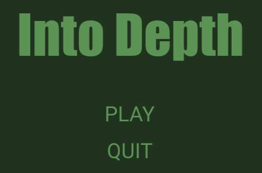
Current title screen using text rendering with the Arial TrueType fonts.

Last month we covered text rendering, which was necessary for getting the scaffolding up that supports the over-arching gameplay loop. We have a title screen, a level select screen, codex screens for seeing information about unlocked heroes and relics, and a level results screen that summarizes what was gained when completing a level. All of these are rudimentary first stabs, but ya got to make it exist first.

A lot happened in the last month, some of which I might cover in future posts. I’m not going to list everything every time, but it is interesting to see just how much stuff goes into making some sort of usable interactive experience when you’re doing a lot from scratch.

  • Added basic hero avatars to display when the hero is selected.
  • Added a tweak file system for rapidly tuning parameters.
  • Expanded the hero struct to include a hero level state to distinguish between in-level heroes and those that have not yet been deployed and those that have exited a level.
  • Added new screens.
  • Generalized my UI panel work to have fancier button logic that properly detects button presses, accounting for when the player clicks elsewhere but releases over the button, or presses down on the button but releases elsewhere.
  • Moved the game interface to simply receive one large memory buffer that the game itself then chops up into whatever smaller allocations and arenas it needs.
  • Introduced local mesh assets that can be directly rendered via the triangle shader from the previous post, used for basic quads and things like the selection outline.
  • Introduced the grid view. More on that in a bit.
  • Added a way to quickly identify which entities are in which cells in the stage, now more necessary due to the grid view.
  • Introduced schedules and simulating consequences up front rather than live.
  • Added the action selection panel and action sub-selection interfaces for hero deployment, move selection, and turn passing. The focus of this blog post.
  • Removed a bunch of earlier code pre-move selection where the active hero would move one tile or perform one action per key press.

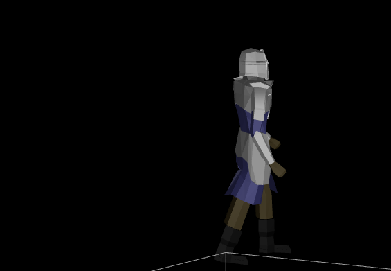
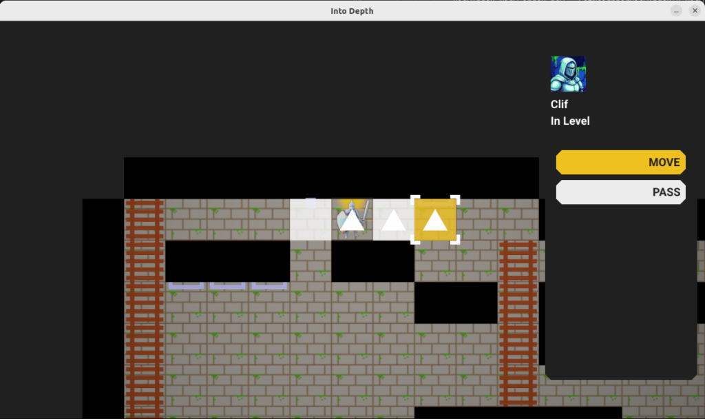
The game now looks like this:

Obviously, all art, layout, UI, etc. is an extremely early first cut and likely not the final version. We do, however, see the basic framework for a game.

Action Panel

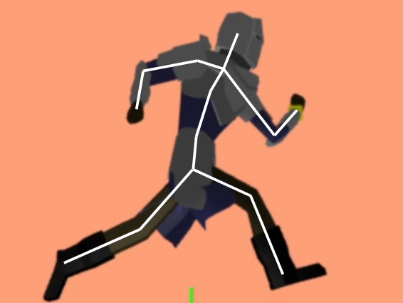
The main thing I want to talk about this week is the fledgling action system, starting with the action panel:

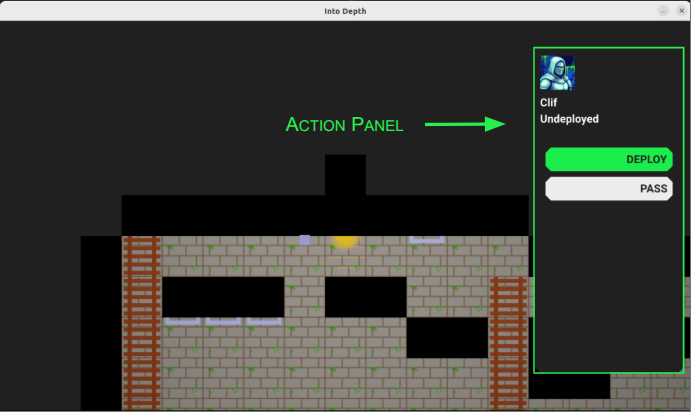
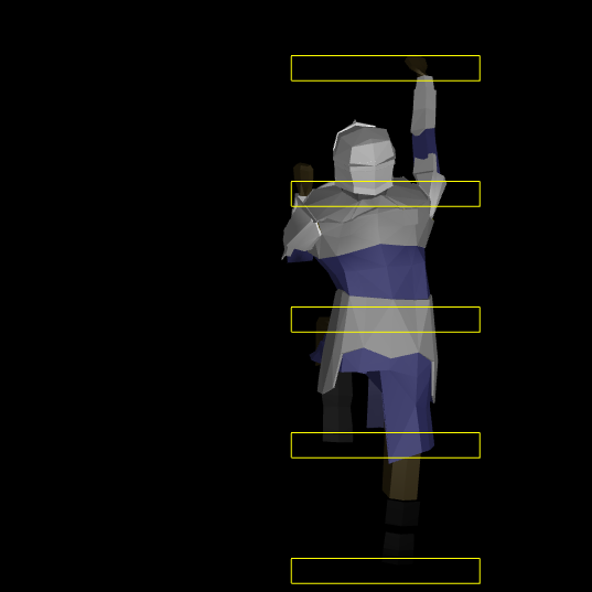
The action panel shows the active hero’s avatar, their name, their level state, and has a series of action buttons.

You’ll notice that the panel has the same color as the background. Eventually, when the field of view includes shadow casting, it should just blend with the shadows. Here is my Google slides mockup of what I’m roughly working toward:

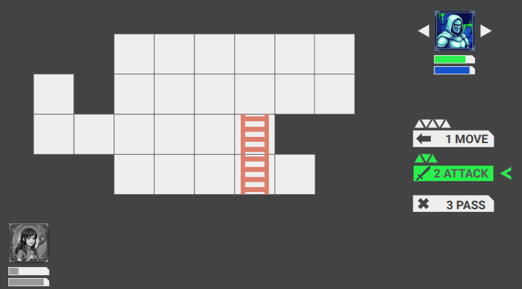
Eventually we’ll see the whole party, along with whatever status bars we need to see, and the actions available to the hero will look fancier. Most notably, I intend to render little equilateral triangles to represent the action points available for various moves. I’m not 100% settled on how that would work, but something like that will happen.

The game loop inside a level tracks which actor is active, and then loops through four states:

  • Generate Actions
  • Select Action
  • Play Schedule
  • Done

The first state is where the game looks at the current state and generates the actions available to the actor. For heroes, these then show up as options in the action panel. The user can then select an action and get access to its dedicated UI, and use that to determine the details.

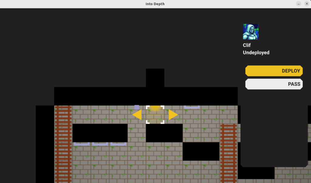
Here we’ve selected the DEPLOY action and we get a user interface for selecting which cell to deploy the hero to.

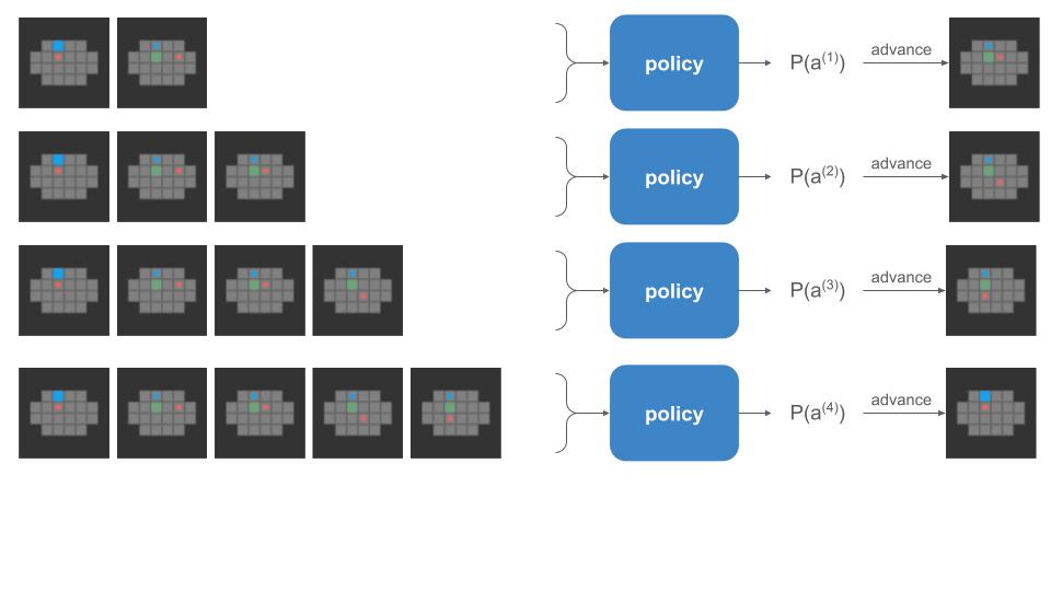
Once the user commits to an action, the action generates a schedule. This is the sequence of events that represent the outcome of the action. For example, passing the turn simply produces an event that moves the game to the next actor. Selecting a move to a cell produces a more complicated schedule that traverses multiple cells in sequence, and may involve posture changes like changing from standing to climbing.

Most importantly, a schedule contains the complete outcome of the action. Previously, if the actor planned to move, I was having the game check live, as the player moved, for triggered events like ending up over an empty shaft and then moving into a falling state. This fragments the logic and makes it harder to test planning and consequence code, as we don’t really know the consequence of an action until it is tediously simulated out over many iterations.

Instead, the schedule does all necessary consequence simulation during construction, and the game then just needs to play that out until it has completed. Given that we have the schedule, it is also quite easy to undo the entire action without having to figure out some weird reverse simulation.

This doesn’t look terribly complicated to implement, but it is actually the system that flummoxed me the most in my previous project attempt, particularly when it came to changing which actions were available based on the actor’s equipment and in enabling undo. I am much happier with how this latest rendition is set up.

The schedule is, at its core, just a DAG of events stored in a topological order:

struct Schedule {
    // Events are in a topological order
    u16 n_timeline;
    Event* timeline; // allocated on the Active linear allocator

    // The net outcome.
    u16 n_outcome;
    Event* outcomes; // allocated on the Active linear allocator

    // The opposite of the net outcome, since events are not inherently reversible.
    u16 n_undo;
    Event* undos; // allocated on the Active linear allocator
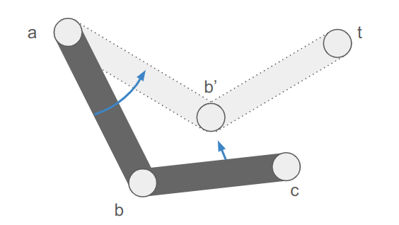
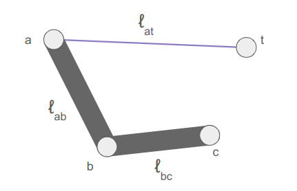
};

The schedule contains the full timeline, plus a compressed net outcome that only contains the events necessary to encode the overall delta. For something like a pass action, the timeline and the outcome are the same. For a move, where the actor traverses multiple cells, the timeline contains the sequence of cell traversals but the outcome only contains one cell change – from source to dest.

The schedule also contains the set of events needed to undo the action. This is very similar to the outcome, just reversed. The game events don’t all contain the information necessary to be reversed, so we construct the undo events separately.

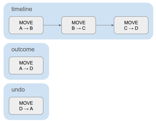
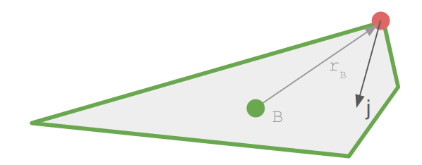
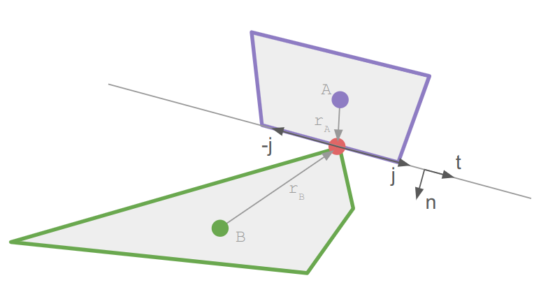
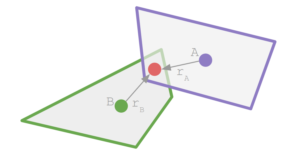
A simple schedule for moving a hero. The timeline contains multiple cell transitions, but the outcome and undo each consist of a single event.

Events are small, composable game state deltas:

struct Event {
    u16 index;  // The event's index in the schedule. (Events are in a topological order)
    u16 beat;   // The beat that this event should be executed on. Events sharing a beat happen concurrently.
    EventType type;

    union {
        EventEndTurn end_turn;
        EventSetHeroLevelState set_hero_level_state;
        EventMove move;
        EventSetCellIndex set_cell_index;
        EventSetFacingDir set_facing_dir;
        EventSetHeroPosture set_hero_posture;
        EventAttachTo attach_to;
        EventOnBelay on_belay;
        EventOffBelay off_belay;
        EventHaulRope haul_rope;
        EventLowerRope lower_rope;
        ... etc.
    };
};

Each event knows its event type and then contains type-specific data. This is a pretty straightforward way to interleave them without annoying object-oriented inheritance code.

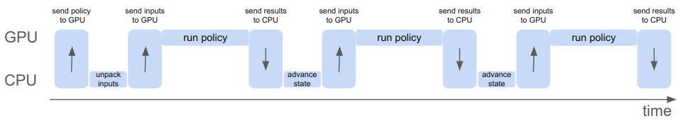
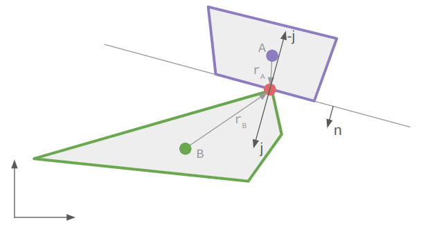
Events also contain beats. The game logic is discrete, and in order to have events run concurrently, we store them in the same beat:

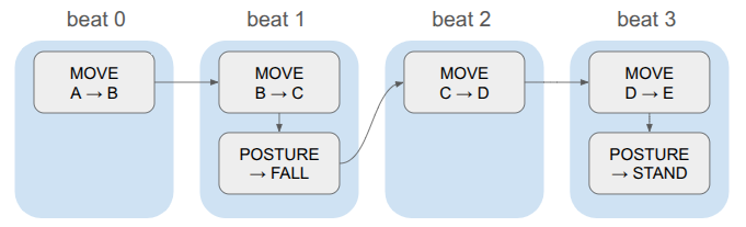
Whenever we advance a beat, we apply all events in that beat and trigger any animations or whatnot and use that to determine how long to wait until we start the next beat. This keeps the event system clean (it doesn’t need to know how long a given animation will take, or even what animation is associated with an event), and gives us one centralized place for triggering animations and sounds.

When the schedule is fully played out, the game enters the done state and checks to see if the level is done. If not, it goes back to action generation.

The state for active levels thus includes the core game state (the stage), which actor’s turn it is, the active schedule (if any), the schedule playback state (event index, time in beat), and data for all of this turn’s actions:

struct ScreenState_Active {
    // The active playable area and the entities in it.
    Stage stage;

    // Stores data for the active actor's turn.
    Turn turn;

    // Stores the events that are scheduled to run.
    Schedule schedule;

    // The playback state of the schedule.
    PlaybackState playback_state;

    // The index of the active actor.
    int i_actor = 0;
    int i_actor_next;

    // Where we allocate the action data.
    // This allocator is only reset when actions are regenerated.
    LinearAllocator action_allocator;
};

Pretty clean when it comes down to it.

The Turn contains the actions generated for the current actor. Each action has a name, which then makes it easy to render the buttons for the actions in the action panel.

Actions

An action is a discrete state change available to an actor, such as passing the turn, moving through the environment, or attacking another actor. The available actions depend on the game state — an actor that is not yet deployed has a deploy action but no move action, and an actor with a bow should get an attack action with a ranged UI whereas an actor with a sword can only select the tiles within melee range.

To handle these things flexibly, actions have methods that can be specialized on a per-action basis. In modern C++, one would probably use objects and inheritance to implement a bunch of action subclasses. I am avoiding classes and am not using inheritance at all, so instead we have a basic struct with some function pointers:

// A function pointer called to run the action UI for the action,
// once the action has been selected in the menu.
typedef void (*FuncRunActionUI)(GameState* game, RenderCommandBuffer* command_buffer, void* data, const AppState& app_state);

// A function pointer for a method that determines whether the action was committed.
typedef bool (*FuncIsActionCommitted)(const void* data);

// A function pointer for a method that builds a schedule from the action.
typedef bool (*FuncBuildSchedule)(GameState* game, void* data);

struct Action {
    char name[16]; // null-terminated

    // The key to press to perform this action
    char shortkey;

    // Data associated with the action, specialized per action type
    void* data;

    // Function pointers
    FuncRunActionUI run_action_ui;
    FuncIsActionCommitted is_action_committed;
    FuncBuildSchedule build_schedule;
};

We use the action name when displaying its button in the action panel, and its shortkey is available if the user doesn’t want to have to click the button with the mouse.

Each action also has a void* data member, which can be populated when the action is created and then used in the member functions. We’ll see an example of that shortly.

Generating the available actions is conceptually straightforward; just run a method for every action in the game that checks if that action is available, and if it is, allocates it, constructs it, and adds it to the action list:

void GenerateActions(GameState* game, const Hero& hero) {
    Turn& turn = game->screen_state_active.turn;
    turn.n_actions = 0;
    turn.i_action_selected = -1;

    if (MaybeGenerateAction_Deploy(&turn.actions[turn.n_actions], game, hero)) {
        turn.n_actions++;
    }
    if (MaybeGenerateAction_Move(&turn.actions[turn.n_actions], game, hero)) {
        turn.n_actions++;
    }
    if (MaybeGenerateAction_Pass(&turn.actions[turn.n_actions], game, hero)) {
        turn.n_actions++;
    }
    ...
}

This may seem too simple, but I think it is actually quite an advantage. I had previously been considering having various pieces of equipment be responsible for determining which actions they are associated with, and then having a way to store that metadata on the equipment, save it to disk, etc. Messy! Instead, I can just run all of these methods, every time, and if any require specific equipment, they can check for it and just quickly return false if it isn’t there.

Every action currently requires at least four methods: action generation, running the action-specific UI, a simple method that determines whether the user committed to the action, and a schedule generation. For the simple pass action, this doesn’t even need the void* data member:

// ------------------------------------------------------------------------------------------------
bool MaybeGenerateAction_Pass(Action* action, GameState* game, const Hero& hero) {

    strncpy(action->name, "PASS", sizeof(action->name));
    action->shortkey = 'p';
    action->run_action_ui = RunActionUI_Pass;
    action->is_action_committed = IsActionCommitted_Pass;
    action->build_schedule = BuildSchedule_Pass;

    return true;
}

// ------------------------------------------------------------------------------------------------
void RunActionUI_Pass(GameState* game, RenderCommandBuffer* command_buffer, void* data, const AppState& app_state) {
    // Nothing to do here.
}

// ------------------------------------------------------------------------------------------------
bool IsActionCommitted_Pass(const void* data) {
    return true;
}

// ------------------------------------------------------------------------------------------------
bool BuildSchedule_Pass(GameState* game, void* data) {
    ScreenState_Active& active = game->screen_state_active;

    // Build the schedule, which consists just of an end turn action.
    Schedule* schedule = &(game->screen_state_active.schedule);
    
    schedule->n_timeline = 1;
    schedule->timeline = (Event*)Allocate(&(active.action_allocator), sizeof(Event));
    ASSERT(schedule->timeline != nullptr, "BuildSchedule_Pass: Failed to allocate timeline!");
    
    CreateEventEndTurn(schedule->timeline, /*index=*/0, /*beat=*/0);

    // The outcome is the same.
    schedule->n_outcome = 1;
    schedule->outcomes = schedule->timeline;

    // The undo action: TODO

    return true;
}

The deploy action is more involved, and it does allocate a custom data struct:

struct DeployActionData {
    // List of legal entry cells for the hero.
    u16 n_entries;
    CellIndex entries[STAGE_MAX_NUM_ENTRIES];

    // The index of the entry we are looking at.
    int targeted_entry;

    // Whether the entry has been selected.
    bool entry_selected;
};

// ------------------------------------------------------------------------------------------------
void InitActionData_Deploy(DeployActionData* data) {
    data->n_entries = 0;
    data->targeted_entry = 0;
    data->entry_selected = false;
}

// ------------------------------------------------------------------------------------------------
bool MaybeGenerateAction_Deploy(Action* action, GameState* game, const Hero& hero) {

    if (hero.level_state != HERO_LEVEL_STATE_UNDEPLOYED) {
        // Hero does not need to be deployed
        return false;
    }

    ScreenState_Active& active = game->screen_state_active;
    const Stage& stage = active.stage;
    
    // Allocate the data for the action
    action->data = Allocate(&(active.action_allocator), sizeof(DeployActionData));
    DeployActionData* data = (DeployActionData*)action->data;
    InitActionData_Deploy(data);

    // Run through all stage entries and find the valid places to deploy
    for (u16 i_entry = 0; i_entry < stage.n_entries; i_entry++) {
        CellIndex cell_index = stage.entries[i_entry];
        
        ASSERT(!IsSolid(stage, cell_index), "Entry cell is solid!");

        // Ensure that the cell is not occupied by another hero
        if (IsHeroInCell(stage, cell_index)) {
            continue;
        }

        // Add the entry.
        data->entries[data->n_entries++] = cell_index;
    }

    if (data->n_entries == 0) {
        // No valid entries
        return false;
    }
    
    
    strncpy(action->name, "DEPLOY", sizeof(action->name));
    action->shortkey = 'd';
    // action.sprite_handle_icon = // TODO
    action->run_action_ui = RunActionUI_Deploy;
    action->is_action_committed = IsActionCommitted_Deploy;
    action->build_schedule = BuildSchedule_Deploy;

    return true;
}

// ------------------------------------------------------------------------------------------------
void RunActionUI_Deploy(GameState* game, RenderCommandBuffer* command_buffer, void* data, const AppState& app_state) {
    
    DeployActionData* action_data = (DeployActionData*)data;

    const TweakStore* tweak_store = &game->tweak_store;
    const f32 kSelectItemFlashMult = TWEAK(tweak_store, "select_item_flash_mult", 2.0f);
    const f32 kSelectItemReticuleAmplitude = TWEAK(tweak_store, "select_item_reticule_amplitude", 0.25f);
    const f32 kSelectItemFlashAlphaLo = TWEAK(tweak_store, "select_item_flash_alpha_lo", 0.1f);
    const f32 kSelectItemFlashAlphaHi = TWEAK(tweak_store, "select_item_flash_alpha_hi", 0.9f);
    const f32 kSelectItemArrowOffsetHorz = TWEAK(tweak_store, "select_item_arrow_offset_horz", 1.0f);
    const f32 kSelectItemArrowScaleLo = TWEAK(tweak_store, "select_item_arrow_scale_lo", 1.0f);
    const f32 kSelectItemArrowScaleHi = TWEAK(tweak_store, "select_item_arrow_scale_hi", 1.0f);

    // TODO: This is probably lagged by one frame.
    const glm::mat4 clip_to_world = CalcClipToWorld(command_buffer->render_setup.projection, command_buffer->render_setup.view);
    const glm::vec2 mouse_world = CalcMouseWorldPos(app_state.pos_mouse, 0.0f, clip_to_world, app_state.window_size);

    bool deploy_hero_to_target_cell = false;

    // Set the hero's location to one tile over the entry we are looking at.
    // This is a hacky way to handle the fact that the hero is not in the level yet

    // and that the camera is centered on the hero
    ScreenState_Active& active = game->screen_state_active;
    Hero* hero = active.stage.pool_hero.GetMutableAtIndex(active.i_actor);
    const CellIndex cell_index = action_data->entries[action_data->targeted_entry];
    MoveHeroToCell(&active.stage, hero, {cell_index.x, (u16)(cell_index.y + 1)});
    hero->offset = {0.0f, 0.0f};

    // Render the entrance we are currently looking at.
    {
        const f32 unitsine = UnitSine(kSelectItemFlashMult * game->t);

        RenderCommandLocalMesh& local_mesh = *GetNextLocalMeshRenderCommand(command_buffer);
        local_mesh.local_mesh_handle = game->local_mesh_id_quad;
        local_mesh.screenspace = false;
        local_mesh.model = glm::translate(glm::mat4(1.0f), glm::vec3(0.0f, -1.0f, RENDER_Z_FOREGROUND));
        local_mesh.color = kColorGold;
        local_mesh.color.a = Lerp(kSelectItemFlashAlphaLo, kSelectItemFlashAlphaHi, unitsine);

        {
            RenderCommandLocalMesh& reticule = *GetNextLocalMeshRenderCommand(command_buffer);
            reticule.local_mesh_handle = game->local_mesh_id_corner_brackets;
            reticule.screenspace = false;
            reticule.model = glm::translate(glm::mat4(1.0f), glm::vec3(0.0f, -1.0f, RENDER_Z_FOREGROUND + 0.1f));
            reticule.model = glm::scale(reticule.model, glm::vec3(unitsine * kSelectItemReticuleAmplitude + 1.0f));
            reticule.color = kColorWhite;
        }

        // Run button logic on the targeted entry.
        const Rect panel_ui_area = {
                .lo = glm::vec2(- 0.5f, - 1.5f),
                .hi = glm::vec2(+ 0.5f, - 0.5f)};
        const UiButtonState button_state = UiRunButton(&game->ui, panel_ui_area, mouse_world);

        if (button_state != UiButtonState::NORMAL) {
            local_mesh.color.x = Lerp(local_mesh.color.x, kColorWhite.x, unitsine);
            local_mesh.color.y = Lerp(local_mesh.color.y, kColorWhite.y, unitsine);
            local_mesh.color.z = Lerp(local_mesh.color.z, kColorWhite.z, unitsine);
        }

        if (button_state == UiButtonState::TRIGGERED) {
            deploy_hero_to_target_cell = true;
        }
    }

    bool pressed_left = IsNewlyPressed(app_state.keyboard, 'a');
    bool pressed_right = IsNewlyPressed(app_state.keyboard, 'd');

    // Render two arrow-like triangles that let us switch between options.
    {
        const f32 unitsine = UnitSine(game->t);
        const f32 scale = Lerp(kSelectItemArrowScaleLo, kSelectItemArrowScaleHi, unitsine);

        const glm::vec2 halfdims = glm::vec2(0.433f * scale, 0.5f * scale); // NOTE: Rotated

        { // Left triangle
            const glm::vec2 pos = glm::vec2(-kSelectItemArrowOffsetHorz, -1.0f);
            
            const Rect panel_ui_area = {
                    .lo = pos - halfdims,
                    .hi = pos + halfdims};
            const UiButtonState button_state = UiRunButton(&game->ui, panel_ui_area, mouse_world);

            RenderCommandLocalMesh& local_mesh = *GetNextLocalMeshRenderCommand(command_buffer);
            local_mesh.local_mesh_handle = game->local_mesh_id_triangle;
            local_mesh.screenspace = false;
            local_mesh.model =
            glm::scale(
                glm::rotate(
                    glm::translate(glm::mat4(1.0f), glm::vec3(pos.x, pos.y, RENDER_Z_FOREGROUND)),
                    glm::radians(90.0f),
                    glm::vec3(0.0f, 0.0f, 1.0f)
                ),
                glm::vec3(scale, scale, 1.0f)
            );
            local_mesh.color = kColorGold;

            if (button_state != UiButtonState::NORMAL) {
                local_mesh.color = glm::mix(local_mesh.color, kColorWhite, unitsine);
            }

            // Check for pressing the button.
            if (button_state == UiButtonState::TRIGGERED) {
                pressed_left = true;
            }
        }
        { // Right triangle
            const glm::vec2 pos = glm::vec2(kSelectItemArrowOffsetHorz, -1.0f);
            
            const Rect panel_ui_area = {
                    .lo = pos - halfdims,
                    .hi = pos + halfdims};
            const UiButtonState button_state = UiRunButton(&game->ui, panel_ui_area, mouse_world);

            RenderCommandLocalMesh& local_mesh = *GetNextLocalMeshRenderCommand(command_buffer);
            local_mesh.local_mesh_handle = game->local_mesh_id_triangle;
            local_mesh.screenspace = false;
            local_mesh.model = 
            glm::scale(
                glm::rotate(
                    glm::translate(glm::mat4(1.0f), glm::vec3(pos.x, pos.y, RENDER_Z_FOREGROUND)),
                    glm::radians(-90.0f),
                    glm::vec3(0.0f, 0.0f, 1.0f)
                ),
                glm::vec3(scale, scale, 1.0f)
            );
            local_mesh.color = kColorGold;

            if (button_state != UiButtonState::NORMAL) {
                local_mesh.color = glm::mix(local_mesh.color, kColorWhite, unitsine);
            }

            // Check for pressing the button.
            if (button_state == UiButtonState::TRIGGERED) {
                pressed_right = true;
            }
        }
    }


    // Process the presses, which can come from keys or clicking the arrows.
    if (pressed_left) {
        CircularDecrement(action_data->targeted_entry, (int)action_data->n_entries);
    } else if (pressed_right) {
        CircularIncrement(action_data->targeted_entry, (int)action_data->n_entries);
    }

    if (deploy_hero_to_target_cell) {
        action_data->entry_selected = true;
    }
}

// ------------------------------------------------------------------------------------------------
bool IsActionCommitted_Deploy(const void* data) {
    const DeployActionData* action_data = (DeployActionData*)data;
    return action_data->entry_selected;
}

// ------------------------------------------------------------------------------------------------
bool BuildSchedule_Deploy(GameState* game, void* data) {
    ScreenState_Active& active = game->screen_state_active;

    const Hero* hero = active.stage.pool_hero.GetAtIndex(active.i_actor);
    const CellIndex src = hero->cell_index;
    const CellIndex dst = {src.x, (u16)(src.y - 1)};

    // Build the schedule, which changes the hero's level state and moves them to the entry (1 cell down).
    Schedule* schedule = &(game->screen_state_active.schedule);
    
    {
        schedule->n_timeline = 2;
        schedule->timeline = (Event*)Allocate(&(active.action_allocator), schedule->n_timeline * sizeof(Event));
        ASSERT(schedule->timeline != nullptr, "BuildSchedule_Deploy: Failed to allocate timeline!");
        
        CreateEventSetHeroLevelState(schedule->timeline, /*index=*/0, /*beat=*/0, hero->id, HERO_LEVEL_STATE_IN_LEVEL);
        CreateEventMove(schedule->timeline + 1, /*index=*/1, /*beat=*/0, hero->id, Direction::DOWN, src, dst);
    }

    // The outcome is the same.
    schedule->n_outcome = 1;
    schedule->outcomes = schedule->timeline;

    // Undo: TODO

    return true;
}

Move Actions

The move action is significantly more complicated than the deploy or pass actions.

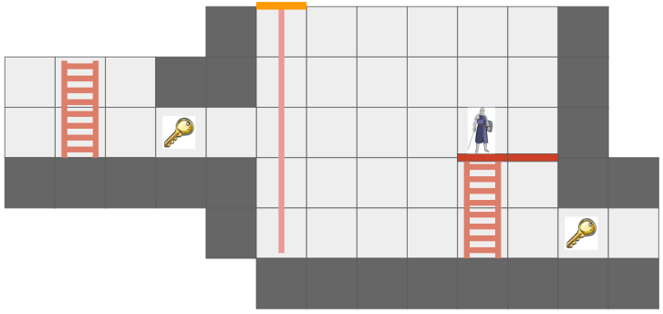
The move action highlights all valid target cells, allowing the player to select one to move to. Once selected, the shortest path to that cell is taken by the hero, and all consequences are simulated (e.g. falling, triggering a trap) and built into a schedule.

The move action UI, which here has three valid target cells (since falling ends the search). The tile under the mouse cursor is highlighted in yellow, has square angle brackets, and the shortest path is shown as a trail of equilateral triangles.

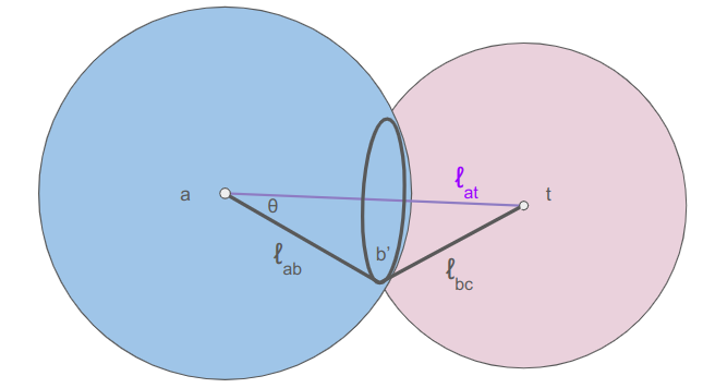
In order to support these features, the move action logic needs to know what the reachable cells are and what the shortest paths to them are. This is achieved by running Dijkstra’s algorithm from the actor’s initial state. The state space is not merely cell positions, but also includes the actor’s facing direction and their posture (standing, on ladder, etc.).

There is one additional point of complication, and that is that we want this game to only reason about cells that are visible from the hero’s current vantage point, and we eventually want to support non-Euclidean connections like portals:

In this mockup, the key is visible twice because the hallway has a portal loop-back connection.

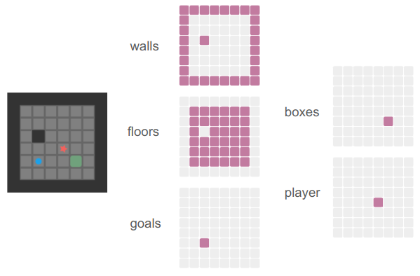
In order to achieve this, we introduce a new representation of the level geometry visible to an actor, the GridView:

struct GridView {
    // The grid tile the view is centered on
    CellIndex center;

    CellIndex cell_indices[GRID_VIEW_MAX_X][GRID_VIEW_MAX_Y];
    u8 flags[GRID_VIEW_MAX_X][GRID_VIEW_MAX_Y];
};

This view has a finite size, much smaller than the overall level grid, that is big enough to fit the screen. The view is always centered on an actor, and the cells in the view are then indices into the cells in the underlying level grid. If a level grid cell is connected by a non-Euclidean portal to another cell, the view can just index into the correct cells on either side of the portal. Constructing the grid view is a straightforward breadth-first search from the center tile.

Note: I am actually temporarily making this simpler than it really is. To do this properly, we’ll need a fancier data structure that is not a grid but can handle sectors, because one view cell may actually contain view sectors of multiple level cells:

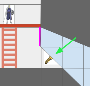
This view cell is visible twice, once with a cell containing a key, with this portal (magenta) set up.

We thus run Dijkstra’s algorithm in this grid view, starting from the center cell where the actor is. The same cell may be visible multiple times in the grid view, and we will correctly be able to route to that cell via multiple paths.

The search assigns a cost for each state change, and only searches up to a maximum cost. Very soon, actors will have action points to spend per turn, and it won’t be possible to move further than are affordable given the action points currently available.

The move action custom data struct is:

struct MoveActionData {
    // We can only ever move to a visible tile, so for now, we can
    // just allocate a grid's worth of potential targets.

    // The cheapest cost to reach each move state.
    u16 costs[GRID_VIEW_MAX_X][GRID_VIEW_MAX_Y][/*num directions=*/2][kNumHeroPostures];

    // The parent state on the shortest path that arrives at the given state.
    // I.E., if [1][2][LEFT][STANDING] contains {2,2,LEFT,STANDING}, then we took a step over.
    // The root state points to itself.
    MoveState parents[GRID_VIEW_MAX_X][GRID_VIEW_MAX_Y][/*num directions=*/2][kNumHeroPostures];

    // Used to track whether a view cell has been visited.
    u32 visit_frame;
    u32 visits[GRID_VIEW_MAX_X][GRID_VIEW_MAX_Y];
    
    ViewIndex view_index_target;  // Target view cell index for the move.
    bool entry_selected;
};

Having completed the search, we are able to render all reachable tiles, render a reticle over the cell the user’s mouse is over, and if the cell is reachable, we can backtrack over the cell’s parents to render the cells traversed to get there. (Since states include more than just cell changes, and we don’t want to render multiple times to the same cell, we also store a u32 visit frame that we can use to mark cells we have rendered to in order to avoid rendering to the same cell multiple times.)

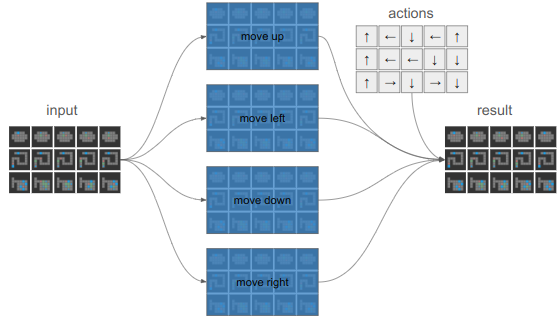
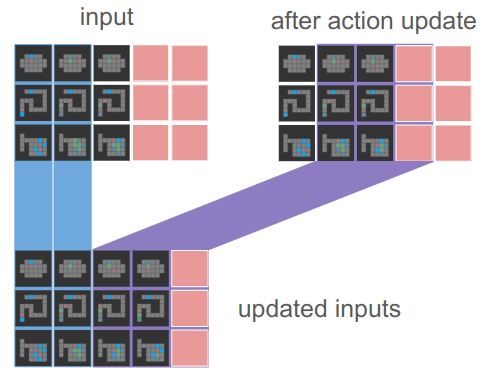
Finally, when the user clicks on a cell to commit the action, we compute the schedule by:

  1. Extracting the shortest path by traversing back to the source node.
  2. Writing the shortest path out one state change at a time.
  3. Simulating consequences (like falling) after every step, and if any consequences do take place, ending the planned schedule there and appending all consequence events.

This process makes a copy of the current state and applies all changes there. Making a copy, while taking memory, has the advantage of not polluting the actual game state and giving us a second Stage to compare the current Stage to in order to get the overall schedule delta.

Conclusion

With the action system in place, the foundation is laid for actual gameplay. Next time, we’ll look at introducing some core entities back in (ropes, buckets, relics) and managing the overall gameplay cycle.

A TrueType Font

TrUeTyPe FoNt

Early in 2025, I had stumbled on concept images of a font with triangular glyphs. Something about it was appealing. I ended up crafting a similar concept, but extending it so that the equilateral triangles could tile together using both upward and downward facing triangles:

The upward and downward facing glyphs for the triangle font, from A to Z.

I was implementing OpenGL font rendering in C++, using Sean Barrett’s TrueType library to load fonts and construct a font atlas. Somewhere in this whole process I decided it would be fun to implement a font I had conceptualized months ago for real, so to speak, as a TrueType font.

TrueType doesn’t support conditional logic for alternating glyph directions like this, so in practice I achieve the effect by making all uppercase characters be upward facing triangles and all lowercase characters be downward facing triangles. The text below is “HeLlO wOrLd”:

HeLlO wOrLd

Having my own game that could load and use the font was helpful for debugging, once the binary was loadable, since I could step through it with a debugger. I also found fontdrop and the hex editor useful.

You can download the font here.

Architecture

There are two fundamental responsibilites: defining the font in memory and serializing it to .ttf:

FontDefinition font = CreateFont();
bool success = ExportFont(&font);

Separating font definition from binary export keeps the system reusable and avoids hard-coded constants leaking into the writer.

CreateFont populates a builder struct:

FontDefinition font;
assert(InitFontDefinition(&font,
    /*units_per_em=*/1000, /*ascent=*/866,
    /*descent=*/0, /*line_gap=*/0,
    /*family_name=*/"TeSsElLaTe",
    /*subfamily_name=*/"Regular",
    /*unique_name=*/"TeSsElLaTe rEgUlAr v1.0",
    /*full_name=*/"TeSsElLaTe rEgUlAr")
  && "Failed to initialize font");

// Create the missing glyph (.notdef) - a simple square
// This glyph is shown when a character is not found in the font
const GlyphId missing_glyph = StartGlyph(&font, /*codepoint=*/0, advance_width, left_side_bearing);
assert(missing_glyph != 0xFFFF && "Failed to start missing glyph");

// Create a square contour with 4 points
assert(StartContour(&font) && "Failed to start contour for missing glyph");
assert(AddPoint(&font, 0, 0, 1) && "Failed to add point 0");
assert(AddPoint(&font, 1000, 0, 1) && "Failed to add point 1");
assert(AddPoint(&font, 1000, 1000, 1) && "Failed to add point 2");
assert(AddPoint(&font, 0, 1000, 1) && "Failed to add point 3");
assert(EndContour(&font) && "Failed to end contour for missing glyph");
assert(EndGlyph(&font) && "Failed to end missing glyph");

The font definition is kept in a truetype.hpp header, along with builder helpers like StartContour and AddPoint. After defining all of the glyphs, we can also add kerning pairs. The default xadvance is set for subsequent equilateral triangles, and I reduce that for pairs that nest together.

ExportFont needs to open a file and write the binary .ttf file. The format consists of a directory listing the tables and their offsets, followed by the tables themselves, padded to 4-bytes. Each table has a checksum, and the data is exported as big-endian (not the default when using fwrite).

I wanted to calculate the table checksums as I wrote to disk to avoid multiple passes over the data. This requirement was realized via a TableWriter struct along with some basic helper methods like WriteU16BE(&writer, value), which exports the value in big-endian and updates the checksum.

struct TableWriter {
    FILE* file;
    u32 checksum;

    u8 word_buffer[4];
    u32 word_buffer_index; // 0-4
};

All WriteXXBE helper methods call down to a void FeedBytesToChecksum(TableWriter* writer, const u8* data, u32 size); method, which appropriately updates the checksum and writes the data to the file.

After writing placeholder values for the directory, the exporter writes all of the tables, in alphabetical order. Each table is written as follows:

// Write cmap table
writer.checksum = 0; // Reset.
TableInfo* table_info = &table_infos[table_index];
table_info->offset = (u32)ftell(writer.file);
table_info->length = WriteCmapTable(&writer, font);
table_info->checksum = writer.checksum;
PadTo4ByteAlignment(&writer);
printf("Wrote %s table (%u bytes, offset %u, checksum 0x%08X)\n",
    table_tags[table_index], table_info->length, table_info->offset, table_info->checksum);
table_index++;

Offset values are captured directly from the file stream as each table is written to disk, enabling a single streaming pass without rewinding or recomputing. Each table has its own WriteXXXXTable method, all of which were kept in a truetype_export.hpp header. This made it easy to iterate on the code.

We then go back and update the table directory. Easy peasy.

Finishing a Vertical Slice

I didn’t know whether the font exporter was working until I was able to load the resulting .ttf file in another program. A vertical slice lets you de-risk binary exporters early. I prioritized this by not immediately defining all glyphs and instead just defined the undefined glyph (.notdef), space, and ‘A’. I implemented the minimum necessary set of TrueType tables that could be loaded by tools like stb_truetype and the browser inspector, helping me confirm correctness before scaling out to A–Z and a-z.

Having a testable vertical slice is essential when coding on any project, whether solo or on a team. Coding without knowing whether your code is working is the same as flying blind. A hex editor provides directional confidence that the structure is forming correctly, but real validation only comes when another program successfully loads the font.

Bugs

Sometimes it is interesting to look at what sorts of issues you run into. Understanding how a process fails tells you where to focus on improvements. The bugs that I spent time investigating were:

  • Glyph alignment (segfault). Each glyph must be word-aligned. IMO, this is not at all obvious from the glyf table documentation.
  • Malformed contours as a result of exporting glyph vertices rather than relative vertices. This was clearly laid out in the documentation.

Image from developer.apple.com.

That was enough to get it working with stb_truetype and my font rendering. In order to get the chrome console to be happy, I additionally had to:

  • Fix the cmap length, which was miscalculated. Code like this is not ideal:
// Calculate subtable length
// Format 4 header: 14 bytes (format, length, language, segCountX2, searchRange, entrySelector, rangeShift)
// Data: reservedPad (2) + 4 arrays of seg_count u16 values (seg_count * 8)
const u16 subtable_length = 14 + 2 + (seg_count * 8);
  • Needing to additionally export the OS/2 table, which includes metrics needed by Windows. The chrome inspector straight up told me to add this.
  • Table alignment (browser load failure). All tables must be 4-byte aligned. This was in the top-level docs:

Image from apple.developer.com.

  • Lastly, kerning was working in my font rendering but not for all characters in chrome. It turned out that almost all of my glyphs start at (0,0), but a few, like ‘d’, did not. Chrome was rendering these further to the left. I had to set the left side bearing for those glyphs.

So two counts of failing to use alignment. Seems like a trend I can be more aware of. Despite chasing binary alignment and metrics, I ran into no memory safety issues like null pointers or leaks — problems typically cited as risks of low-level code.

Initializer Lists

I am trying to write in a Muratori-inspired minimal C++ style. That is, C++ without a lot of the C++ features. Avoid classes, macros, templates, and the standard libraries. Why? Ostensibly because simpler code is sufficient, and then easier to understand and faster to compile / execute. Though doing it because I think it is interesting and I admire people like Casey and attitudes like this one from Chris Wellons is also a perfectly valid reason.

I was able to author everything to adhere to this style, but found that I really did want to use initializer lists to simplify glyph creation:

assert(AddGlyph(&font, 'A', advance_width, left_side_bearing,
        {{A, D, N, O, E, B, C}, {S, L, R}}) && "Failed to add A glyph");

I totally could do that without it:

const GlyphId glyph = StartGlyph(&font, 'A', advance_width, left_side_bearing);
assert(glyph != 0xFFFF && "Failed to start glyph");

assert(StartContour(&font) && "Failed to start contour");
assert(AddPoint(&font, font.units_per_em*A.x, font.units_per_em*A.y, 1) && "Failed to add point");
assert(AddPoint(&font, font.units_per_em*D.x, font.units_per_em*D.y, 1) && "Failed to add point");
assert(AddPoint(&font, font.units_per_em*N.x, font.units_per_em*N.y, 1) && "Failed to add point");
assert(AddPoint(&font, font.units_per_em*O.x, font.units_per_em*O.y, 1) && "Failed to add point");
assert(AddPoint(&font, font.units_per_em*E.x, font.units_per_em*E.y, 1) && "Failed to add point");
assert(AddPoint(&font, font.units_per_em*B.x, font.units_per_em*B.y, 1) && "Failed to add point");
assert(AddPoint(&font, font.units_per_em*C.x, font.units_per_em*C.y, 1) && "Failed to add point");
assert(EndContour(&font) && "Failed to end contour");

assert(StartContour(&font) && "Failed to start contour");
assert(AddPoint(&font, font.units_per_em*S.x, font.units_per_em*S.y, 1) && "Failed to add point");
assert(AddPoint(&font, font.units_per_em*L.x, font.units_per_em*L.y, 1) && "Failed to add point");
assert(AddPoint(&font, font.units_per_em*R.x, font.units_per_em*R.y, 1) && "Failed to add point");
assert(EndContour(&font) && "Failed to end contour");

assert(EndGlyph(&font) && "Failed to end glyph");

You can see why I wanted to save myself the typing.

Unfortunately, in addition to including <initializer_list>, I also ended up including <vector> because I was calling AddGlyph with a transform for all downward facing glyphs:

assert(AddGlyph(&font, 'f', advance_width, left_side_bearing,
        ReflectToDownwardGlyph({{A,B,F,J,N,U,V,S,G,C}}, t))
        && "Failed to add f glyph");

Unfortunately, I couldn’t have ReflectToDownwardGlyph modify an initializer list and produce a new one. Instead, I had to return an std::vector. Oh well.

There probably are reasonable ways to do this in an minimal style. If you happen to know, please send me a message!

Conclusion

It was fun to work on a self-contained, somewhat artistic project. I got a chance to try both the Cursor and Antigravity agentic IDEs, both of which worked quite well.

I’m not sure that I’ll be able to author posts monthly, but hopefully this is a good start to returning to my creative outlet. Happy Holidays!

Hiatus

After several years of monthly posts, I am stepping back from the blog for a bit. We’re having a baby!

In the mean time, please stay creative, engaged, and curious.

Grandmother Cells and Black Swans

When I was first learning about deep learning, the teacher brought up an issue with image classifiers and black swans. I would call this the black swan problem, but it turns out that has a related but different meaning, so let’s go with swan classifier generalization problem. It goes like this:

If you train a classifier to identify objects in images, and one of those categories is swans, that classifier will tend to be training exclusively or predominantly on white swans. At deployment it is likely to misclassify images of Australian black swans.

This isn’t all that surprising. Generalization in deep learning is hard.

What is surprising is:

Most humans familiar with swans would be able to recognize an Australian black swan as a swan.

In other words, humans are good at generalization and are able to do it better than many of our traditional deep learning tools, at least in comparison to ImageNet and other, older, deep image classifiers.

This post is an exploration into deep learning, classification, and generalization, and about why I think feature embeddings go a long way to building a better knowledge representation. None of this is particularly new or insightful – I just find it useful to work it out and tie it all together.

Grandmother Cells

A deep image classifier takes as input an image and produces as output a softmax distribution over a discrete set of categories:

Conventional knowledge is that deeper levels reason about more sophisticated, higher-level features. Very early convolutional layers typically only have access to small neighborhoods of pixels, so learn local features like edge detections and textures. Deeper layers might piece together larger structures like a bird beak or ripples in a lake. Finally, all of this information is brought together to produce the final classification.

Under such an approach, you literally have one, single neuron at the end responsible for firing when it thinks the image has a swan. The more intensely its output value, the more confident the swan prediction.

There have historically been two opposing views on the relationship between brains and behavior — the localist view that specific brain regions are responsible for specific behaviors, and the holistic view that neural activity is spread out throughout the nervous system. A critic of the localist view might think it absurd that there is a single neuron somewhere in your head that fires over the concept of “Grandmother”.

A grandmother cell is just that — a neuron exclusively dedicated to one high-level but specific concept. (Funny enough, there was a lot of hubbub in 2005 about recordings that suggested that a single neuron had been found that triggers only for Jennifer Aniston.)

By and large, researchers do not believe that the best way to represent knowledge is through a 1:1 representation such as grandmother cells. As such, it may not come as a surprise when a traditional convolutional deep image classifier like ImageNet struggles to classify black swans.

Sparse Encodings

A traditional image classifier is structured to prefer sparse outputs. A confident prediction should produce a high value in the appropriate category and very low values elsewhere:

If the model is uncertain, it is forced to make the appropriate trade-off to assigning some probability mass to the other potential categories. That might mean assigning some likelihood to other black birds:

This sort of representation might be convenient for the output of a classifier, but it isn’t all that useful for reasoning. If I am trying to think about what it means for an object to be a swan, I don’t want to simply know it is a swan, I want to think about where I might find it (e.g. on a lake), what it might do (e.g. honk at me), and sure, what it looks like (e.g. tends to be white-feathered).

A reasoning network that receives the fact that there is a swan would thus have to unpack this discrete bit of knowledge into these myriad facts:

Worse yet, if you have an uncertain input, you have to unpack all contributors and figure out how to combine them:

Working directly with the discrete bit of knowledge is fragile. If \(P(\text{swan})\) is low, then the network just can’t associate the object to a swan. However, if we’re working with the distributed properties and associations of a swan, its a whole lot easier to get to swan if one property (color), is unusual.

The third thing going on here is that sparse representations don’t use the state space as efficiently. If my reasoning network receives a \(128-\) dimensional vector, and we’re working with one-hot encodings where everything but one dimension is zero, then we can only represent 128 different concepts. In contrast, if we’re willing to use the whole state space, we can represent more or less any number of concepts.

A 2D embedding for the MNIST digits. The left-side shows how digits are mapped to the embedding, and the right shows how samples from the space produce digit images. Images from Algorithms for Decision Making.

Discrete representations are thus hard to work with, fragile, and wasteful.

Transformer Embeddings

You might think that the transformer model suffers from this same problem of discrete reasoning, as they operate on sequences of one-hot tokens. However, these discrete tokens are immediately mapped to a rich embedding vector:

The encoder literally has a separate high-dimensional embedding vector for each discrete token. If we have a vocabulary of \(m\) unique tokens and an \(n\)-dimensional embedding space, then our embeddings are given by an \(n \times m\) matrix. Multiplying by the one-hot token extracts the embedding vector:

\[\boldsymbol{e}^{(i)} = \begin{bmatrix}\boldsymbol{e}^{(1)}, \boldsymbol{e}^{(2)}, \cdots \boldsymbol{e}^{(i)}, \cdots, \boldsymbol{e}^{(m)} \end{bmatrix} \begin{bmatrix}0 \\ 0 \\ \vdots \\ 1 \\ \vdots \\ 0\end{bmatrix}\]

Transformers learn what values to assign to these embedding vectors. As such, they can pack a lot of meaning into those \(n\) dimensions, far more than would be used if it was stuck operating on \(m\) discrete categories.

I talk about transformers in Transformers, How and Why They Work, but gloss over what these embedding vectors really give us. Transformer layers are best thought of as taking the input embedding vectors, which each point in some direction, and incrementally rotating them to point in other directions. (There’s a great video of this by 3Blue1Brown.)

Keep in mind that these are actually very high-dimensional feature spaces.

The initial embedding value is the one the raw token is associated with. The final embedding value is the output of all of the transformer layers, right before a final set of affine layers to go from an \(n\)-dimensional embedding to an \(m\)-dimensional set of logits for the next token.

That means:

  • the final embedding should have of the information for predicting the next token
  • the initial embedding value have the superposition of all meanings the general token

Those are two very different things – hence the need for all those transformer layers and incremental updates.

A final embedding that predicts the next word in “the cat sat on the” needs to capture all the things that a cat might sit on (e.g. laps, mats), as well as adjectives of places cats might sit (e.g. warm laps), and who knows what else people append to that sentence. There is no way that we could capture that superposition of meaning with only \(m\) discrete options.

Interestingly, an initial embedding value also needs to represent a superposition of concepts. The embedding for “mat” for example, might mean a nice place for a cat to sit in one context, but could also be a large concrete slab, or a thick wad of hair.

That means the initial embedding for “mat” should lie in a similar direction as those other concepts. At the very least, it would likely have subcomponents of its \(n\)-dimensional feature space that lie in similar directions. A part of “mat” and “slab” will align for the meaning they share, and likely a different part of “mat” and “matted hair” would align for the meaning those two words share.

This all shows how Transformers are able to assign juxtapositions of meanings using embedding vectors. It can do this in part because the continuous feature space allows for cramming a lot of meanings into the same number of dimensions, allows for smoothly interpolating between meanings, and because a single direction can be made up for sub-directions that have their own meanings. That is exactly what we’re looking for when we want to predict a black swan when we know we need a word for a feathered creature with a big beak on a lake that honks and happens to be colored black.

Why do Transformers learn all this? Because they have to in order to predict the next token accurately. Language is incredibly rich and carries all of these layered meanings.

More Holistic than Local?

One of the big takeaways for me is that knowledge representation using transformer-like dense embeddings is able to pack in and superimpose many concepts, and ends up being less fragile as a result. If enough of the concepts point to a swan, we can still deduce that we need a swan.

I am not a neuroscientist, but I find it highly likely that true grandmother neurons are quite rare. Instead, meaning is more likely to be found packed into subspaces represented by groups of neural firing patterns.

Similarly, I am reminded of writing software for robotics applications. If you’re writing code yourself, then you’re likely basing your reasoning on a comparatively small set of concepts. Take a sidewalk delivery robot for example. A reasonable programmer might try to enforce that the sidewalk delivery robot never cross a light on red. However, said reasonable programmer might get sad when they run into a case where an intersection is under construction and the light is red, but the path is open to pedestrians and delivery robots:

The world is a complicated place, and we quickly find that the number of cases our coded heuristics can handle is quite small. We can easily set ourselves up for failure if we code like grandmother cells. At the very least, code that makes declarative statements needs to be very careful to make declarative statements about what it really is judging — whether the contextual scene is appropriate for crossing or not rather than whether the light is red. As we’ve already learned – getting hung up on color is what motivated this blog post in the first place.

Can we rewrite robotics logic to use embedding vectors? Perhaps. Unfortunately, transformer embeddings are fairly inscrutable to anyone other than the transformer. Interpretable machine learning is still a nascent field.

I think transformers are incredible, but I also think some fundamental properties are missing. They don’t really understand the world yet, not really. AI fails in embarrassing ways. We as humans can write code to reason about \(m\) discrete things. We have a much harder time reasoning about all of the overlapping subtleties of the real world.

Conclusion

This post doesn’t really have a decisive answer. In fact, I hope it serves as food for thought.

I think it is worth pondering these questions as we move forward in this bold new world of Software 2.0, where everything is a transformer and we can do more than we ever could before but don’t really understand how it works or just how far it can take us.

I think this is an incredibly exciting time. It seems like we are very close to cracking the nut of “how we think”. Heck, even John Karmack started working on AI because he feels similarly.

There is likely still something to be learned from how the human brain works. It is the reference model that we have, the irrefutable evidence that there are systems that can reliably learn and then reliably perform well on real-world tasks. Intelligences that know that crossing at red when the road is blocked to cars. Intelligences that more-or-less do the right thing, with very few training examples. Those intelligences may not have figured it out just yet, but perhaps by searching more within, they can finally get to the bottom of things.

Coding your own Tools

We’re working on finalizing the 2nd Edition of Algorithms for Optimization. We originally set out to add three new chapters, but in addition to that overhauled most of the book. Its pretty exciting!

These projects are so big, and so long, that you’ll inevitably run into all sorts of new challenges because time has passed, some dependencies are no longer supported, you try to do things better / a different way, or the MIT Press requirements have changed. That last one is the inspiration for this blog post.

I ended up writing some new tooling to support alttext. Short for alternative text for images, alttext is textual content that can be associated with an image and read out to someone using a screen reader. It wasn’t part of the submission materials when we wrote Algorithms for Optimization v1 and Algorithms for Decision Making, but this time around, MIT Press asked that we supply alttext for every figure in a big spreadsheet. New challenge!

Mykel and I are somewhat different when it comes to being textbook authors. Most authors submit large Word documents with disparate images and let the MIT Press team handle the final text layout. Not us. We provide the final printable PDF.

Our setup is quite nice. It is all under source control, we have a ton of control over how everything looks, and we have everything for the book in one place.

When I saw the ask to supply this additional spreadsheet, I instantly became worried that having a separate sheet could cause problems. That sheet needs to be kept in-sync with the textbook — if any figures are added or removed, we want to make sure they are also added or removed from the sheet. The sheet is also a somewhat inconvenient place to write the alttext. Ideally it would be defined in the LaTeX documents, alongside the figure that it describes. Most importantly, we need to know if we’re missing any alttext.

Storing Tests by Code

We already have some nice technology in our textbook-writing workflow that lets us use the algorithms that we present to the reader to both generate figures and author + execute unit tests.

We present our algorithms using Pythontex and algorithm environments:

\begin{algorithm}
\begin{juliaverbatim}
diff_forward(f, x; h=1e-9) = (f(x+h) - f(x))/h
diff_central(f, x; h=1e-9) = (f(x+h/2) - f(x-h/2))/h
diff_backward(f, x; h=1e-9) = (f(x) - f(x-h))/h
\end{juliaverbatim}
\caption{...}
\end{algorithm}

The juliaverbatim blocks get typeset, but they aren’t executed.

We have a script that parses our source files for algorithm blocks and exports the juliaverbatim contents into a big Julia source file belonging to an Alg4Opt.jl Julia package. We can then load this package when executing Pythontex blocks that do execute, for generating our figures.

We have had unit testing since the beginning. When we first wrote Algorithms for Optimization, we had the unit tests in a separate directory, written in the test files for the Alg4Opt.jl Julia package we exported to. That worked, but the tests were written in an entirely different place than the methods. Sound like storing alttext somewhere other than the figures?

We ended up defining a no-op LaTeX environment:

\excludecomment{juliatest}

and then add those after every algorithm block:

\begin{juliatest}
let
for (f,x,∂) in [(x->x, 0.0, 1.0),
(x->x, 1.0, 1.0),
(x->x, 1.0, 1.0),
(x->x^2, 0.0, 0.0),
(x->x^2, 1.0, 2.0),
(x->x^2, -1.0,-2.0)]
@test isapprox(diff_forward(f, x), ∂, atol=1e-6)
@test isapprox(diff_central(f, x), ∂, atol=1e-6)
@test isapprox(diff_backward(f, x), ∂, atol=1e-6)
end
end
\end{juliatest}

We then parse the LaTeX source files in the same way we do for the algorithm blocks, and export the contents of any juliatest block as unit tests.

Storing the tests next to the algorithms makes things a lot nicer.

Pulling Alttext

I decided that I could do something very similar for alttext.

I defined a dummy command that like juliatest does nothing when compiling the book, but lets us put the alttext content into it:

\newcommand{\alttext}[1]{}

We can then use it in the source code to define the alttext alongside the figure:

\caption{
A one-dimensional optimization problem.
Note that the minimum is merely the best in the feasible set---lower points may exist outside the feasible region.
\label{fig:one-d-opt-prob}
\alttext{A line chart with a single undulating curve and an interval
containing a local minimum identified as the feasible set.}
}

I then wrote a script that runs through our source files and finds all figure and marginfigure blocks, and searches for such a command. If it finds it — great, we can pull out the alttext content and export it to that spreadsheet we need. If not, we can print out a warning that that figure (whose \label ID we also extract), is missing alttext. A nice, simple scripted solution.

Expand this to view the full script.

using Printf

mutable struct FigureEntry
    file_index::Int    # Index into chapter files
    line_index_lo::Int # Index into the chapter's lines at which the \begin resides
    line_index_hi::Int # Index into the chapter's lines at which the \end resides
    label::String      # Figure label, as defined by \label command (or empty)
                       # Figures may not have labels if they are in solutions or examples.
    alttext::String    # Alt text, as given by an \alttext command (or empty)
                       # Every figure is expected to have alttext for the final deliverable.
end

function is_start_of_block(str, block)
    return startswith(str, "\\begin{$block}")
end

function is_end_of_block(str, block)
    return startswith(str, "\\end{$block}")
end

function get_files(; chapter_regex::Regex = r"include\{chapter")
    retval = String[]
    for line in readlines("optimization-chapter.tex")
        if occursin(chapter_regex, line)
            m = match(r"chapter/\S*(?=\})", line)
            @assert isa(m, RegexMatch)
            push!(retval, m.match*".tex")
        end
    end
    return retval
end

function find_matching_paren(str::String, starting_index::Int=something(findfirst(isequal('('), str), 0))
    @assert str[starting_index] == '('
    nopen = 1
    i = starting_index
    n = lastindex(str)
    while nopen > 0 && i < n
        i = nextind(str,i)
        nopen += str[i] == '('
        nopen -= str[i] == ')'
    end
    return nopen == 0 ? i : -1
end

"""
Find the text for a label, such as "fig:gradient_descent_rosenbrock" from
\\label{fig:gradient_descent_rosenbrock}

There should only ever be one \\label entry. In the event that there are multiple,
this methods returns the first one.
If no label is found, this method returns an empty string.
"""
function find_label(lines, line_index_lo::Int, line_index_hi::Int)::String
    for line in lines[line_index_lo:line_index_hi]
        m = match(r"\\label\{([a-zA-Z0-9_:\\-]+)\}", line)
        if isa(m, RegexMatch)
            return m[1]
        end
    end
    return ""
end

"""
Find the alttext for a figure, which is contained inside an \\alttext{} command.
There should only ever be one \\alttext entry per figure. In the event that there are multiple,
this methods returns the first one.
If no alttext is found, this method returns an empty string.
"""
function find_alttext(lines, line_index_lo::Int, line_index_hi::Int)::String
    for line in lines[line_index_lo:line_index_hi]
        m = match(r"\\alttext\{([^}]+)\}", line)
        if isa(m, RegexMatch)
            return m[1]
        end
    end
    return ""
end

function pull_figures()
    is_start_of_ignore = str -> is_start_of_block(str, "ignore")
    is_start_of_figure = str -> is_start_of_block(str, "figure")
    is_start_of_marginfigure = str -> is_start_of_block(str, "marginfigure")
    is_start_of_relevant_block = str -> is_start_of_figure(str) || is_start_of_marginfigure(str) || is_start_of_ignore(str)

    figures = FigureEntry[]
    for (file_index, filepath) in enumerate(get_files())
        filename = splitext(splitdir(filepath)[2])[1]

        println("\treading ", filename)
        lines = [replace(line, "\n"=>"") for line in open(readlines, filepath, "r")]

        counter = 0
        i = something(findfirst(is_start_of_relevant_block, lines), 0)
        while i != 0
            block = is_start_of_ignore(lines[i]) ? "ignore" :
                    is_start_of_figure(lines[i]) ? "figure" :
                                                   "marginfigure"
            j = findnext(str -> is_end_of_block(str, block), lines, i+1)

            if block != "ignore"
                label = find_label(lines, i, j)
                alttext = find_alttext(lines, i, j)
                push!(figures, FigureEntry(file_index, i, j, label, alttext))
            end

            i = something(findnext(is_start_of_relevant_block, lines, j), 0)
        end
    end
    return figures
end

# Find all figure and marginfigure blocks
println("Pulling all figures")
figures = pull_figures()
for (i_figure, figure) in enumerate(figures)
    @printf "%3d %2d [%04d:%04d] %s\n" i_figure figure.file_index figure.line_index_lo figure.line_index_hi figure.label
    println("      $(figure.alttext)")
end

n_figures_missing_alttext = sum(fig.alttext == "" for fig in figures)
if n_figures_missing_alttext > 0
    println("MISSING ALT TEXT!")
    files = get_files()
    for (i_figure, figure) in enumerate(figures)
        label_text = figure.label
        if label_text == ""
            label_text = "UNLABELED"
        end
        @printf "%2d %s in %s\n" i_figure figure.label files[figure.file_index]
    end
end

println("")
println("$(length(figures) - n_figures_missing_alttext) / $(length(figures)) figures have labels")
println("Good job!")

The Joy of Coding your own Tools

That’s what this blog post is really about. The fact that you can dig in and code your own solution. We spend so much time coding for big company projects, that it is easy to forget that we can code small, useful things for ourselves.

The coding we did here is not particularly clever, nor particularly difficult, nor particularly large. That isn’t the point. The point is that we had a problem, and we were able to solve it ourselves with software. Our tools of the trade were brought to bear on our own problem.

I don’t often use coding to solve my own problems, but it does happen every so often. I used coding to create placecards for my wedding, for example, and to create the wedding website. I’ve written code to generate .svg files for CNC laser cutters, in order to craft a loved one a nice birthday present. In high school, I wrote a basic notecard program for practicing my French vocab. That one was super useful.

I am a big fan of Casey Muratori of Handmade Hero (and Computer, Enhance!), which gave rise to the handmade movement. The ideas there are very similar — there is joy to be had from building things yourself, and you are smart enough to dive into something and learn how it works.

Anyhow, I think its nice to be reminded of all this from time to time. Happy coding!

Emscripten is Neat

I spent most of December on vacation, so no big post. However, I did learn about Emscripten, a C++ compiler that produces an executable in WebAssembly. I tried it out and have to say, it was remarkably easy to get something up and running.

I made a very simple crossword game. You you can try it out here.

Best on desktop. While it does load in the browser, it is looking for key events, which is really cumbersome on mobile.

This was written with SDL2 and Dear ImGUI.

Compilation is pretty straightforwad. Instead of running gcc <srcs> <libs> you run emcc <srcs> <libs>. The compiler does some magic to reinterpret use of OpenGL with WebGL, and spits out a .wasm binary blob, a .js script that can execute it, and a .html page that runs it all. My game link above is simply to that .html page.

To test it locally without uploading it to a web page, you can simply start a Python server in your dev directory:

python -m http.server

and then open your .html file in the browser:

http://localhost:8000/your_thing.html

I spend a lot of time tinkering with games and other programs in C++, but I’m developing on a Linux machine. As a result, I can’t really share my games with my friends. Emscripten might be a nice way to achieve that.

Happy 2025 everyone. Hope its a good one.

Rollouts on the GPU

Last month I wrote about moving the Sokoban policy training code from CPU to GPU, yielding massive speedups. That significantly shortened both training time and the time it takes to compute basic validation metrics. It has not, unfortunately, significantly changed how long it takes to run rollouts, and relatedly, how long it takes to run beam search.

The Bottleneck

The training that I’ve done so far has all been with teacher forcing, which allows all inputs to be passed to the net at once:

When we do a rollout, we can’t pass everything in at once. We start with our initial state and use the policy to discover where we end up:

The problem is that the left-side of that image, the policy call, is happening on the GPU, but the right side, the state advancement, is happening on the CPU. If a rollout involves 62 player steps, then instead of one data transfer step like we have for training, we’re doing 61 transfers! Our bottleneck is all that back-and-forth communication:

Let’s move everything to the GPU.

CPU Code

So what is currently happening on the CPU?

At every state, we are:

  1. Sampling an action for each board from the action logits
  2. Applying that action to each board to advance the state

Sampling from the actions is pretty straightforward to run on the GPU. That’s the bread and butter of transformers and RL in general.

# policy_logits are [a×s×b] (a=actions, s=sequence length, b = batch size)
policy_logits, nsteps_logits = policy(inputs)

# Sample from the logits using the Gumbel-max trick
sampled_actions = argmax(policy_logits .+ gumbel_noise, dims=1)

where we use the Gumbel-max trick and the Gumble noise is sampled in advance and passed to the GPU like the other inputs:

using Distributions.jl
gumbel_noise = rand(Gumbel(0, 1), size(a, s, b))

Advancing the board states is more complicated. Here is the CPU method for a single state:

function maybe_move!(board::Board, dir::Direction)::Bool
    â–¡_player::TileValue=find_player_tile(board)
    step_fore = get_step_fore(board, dir)

    â–¡ = â–¡_player # where the player starts
    â–© = â–¡ + step_fore # where the player potentially ends up

    if is_set(board[â–©], WALL)
        return false # We would be walking into a wall
    end

    if is_set(board[â–©], BOX)
        # We would be walking into a box.
        # This is only a legal move if we can push the box.
        â—° = â–© + step_fore # where box ends up
        if is_set(board[â—°],  WALL + BOX)
            return false # We would be pushing the box into a box or wall
        end

        # Move the box
        board[â–©] &= ~BOX # Clear the box
        board[â—°] |= BOX # Add the box
    end

    # At this point we have established this as a legal move.
    # Finish by moving the player
    board[â–¡] &= ~PLAYER # Clear the player
    board[â–©] |= PLAYER # Add the player

    return true
end

There are many ways to represent board states. This representation is a simple Matrix{UInt8}, so an 8×8 board is just an 8×8 matrix. Each tile is a bitfield with components that can be set for whether that tile has/is a wall, box, floor, or tile.

Moving the player has 3 possible paths:

  • successful step: the destination tile is empty and we just move the player to it
  • successful push: the destination tile has a box, and the next one over is empty, so we move both the player and the box
  • failed move: otherwise, this is an illegal move and the player stays where they are

Moving this logic to the GPU has to preserve this flow, use the GPU’s representation of the board state, and handle a tensor’s worth of board states at a time.

GPU Representation

The input to the policy is a tensor of size \([h \times w \times f \times s \times b]\), where 1 board is encoded as a sparse \((h = \text{height}) \times (w=\text{width}) \times (f = \text{num features} = 5)\) tensor:

and we have board sequences of length \(s\) and \(b\) sequences per batch of them:

I purposely chose 4-step boards here, but sequences can generally be much longer and of different lengths, and the first state in each sequence is the goal state.

Our actions will be the \([4\times s \times b]\) actions tensor — one up/down/left/right action per board state.

Shifting Tensors

The first fundamental operation we’re going to need is to be able to check tile neighbors. That is, instead of doing this:

â–¡ = â–¡_player # where the player starts
â–© = â–¡ + step_fore # where the player potentially ends up

we’ll be shifting all tiles over and checking that instead:

is_player_dests = shift_tensor(is_players, d_row=0, d_col=1)

The shift_tensor method method takes in a tensor and shifts it by the given number of rows and columns, padding in new values:

We pass in the number of rows or columns to shift, figure out what that means in terms of padding, and then leverage NNlib’s pad_constant method to give us a new tensor that we clamp to a new range:

function shift_tensor(
    tensor::AbstractArray,
    d_row::Integer,
    d_col::Integer,
    pad_value)

    pad_up    = max( d_row, 0)
    pad_down  = max(-d_row, 0)
    pad_left  = max( d_col, 0)
    pad_right = max(-d_col, 0)

    tensor_padded = NNlib.pad_constant(
        tensor,
        (pad_up, pad_down, pad_left, pad_right, 
            (0 for i in 1:2*(ndims(tensor)-2))...),
        pad_value)

    dims = size(tensor_padded)
    row_lo = 1 + pad_down
    row_hi = dims[1] - pad_up
    col_lo = 1 + pad_right
    col_hi = dims[2] - pad_left

    return tensor_padded[row_lo:row_hi, col_lo:col_hi,
                         (Colon() for d in dims[3:end])...]
end

This method works on tensors with varying numbers of dimensions, and always operates on the first two dimensions as the row and column dimensions.

Taking Actions

If we know the player move, we can use the appropriate shift direction to get the “next tile over”. Our player moves can be reflected by the following row and column shift values:

UP = (d_row=-1, d_col= 0)
LEFT = (d_row= 0, d_col=-1)
DOWN = (d_row=+1, d_col= 0)
RIGHT = (d_row= 0, d_col=+1)

This lets us convert the CPU-movement code into a bunch of Boolean tensor operations:

function advance_boards(
    inputs::AbstractArray{Bool}, # [h,w,f,s,b]
    d_row::Integer,
    d_col::Integer)

    boxes  = inputs[:,:,DIM_BOX,   :,:]
    player = inputs[:,:,DIM_PLAYER,:,:]
    walls  = inputs[:,:,DIM_WALL,  :,:]

    player_shifted = shift_tensor(player, d_row, d_col, false)
    player_2_shift = shift_tensor(player_shifted, d_row, d_col, false)

    # A move is valid if the player destination is empty
    # or if its a box and the next space over is empty
    not_box_or_wall = .!(boxes .| walls)

    # 1 if it is a valid player destination tile for a basic player move
    move_space_empty = player_shifted .& not_box_or_wall

    # 1 if the tile is a player destination tile containing a box
    move_space_isbox = player_shifted .& boxes

    # 1 if the tile is a player destination tile whose next one over
    # is a valid box push receptor
    push_space_empty = player_shifted .& shift_tensor(not_box_or_wall, -d_row, -d_col, false)

    # 1 if it is a valid player move destination
    move_mask = move_space_empty

    # 1 if it is a valid player push destination
    # (which also means it currently has a box)
    push_mask = move_space_isbox .& push_space_empty

    # new player location
    mask = move_mask .| push_mask
    player_new = mask .| (player .* shift_tensor(.!mask, -d_row, -d_col, false))

    # new box location
    box_destinations = shift_tensor(boxes .* push_mask, d_row, d_col, false)
    boxes_new = (boxes .* (.!push_mask)) .| box_destinations

    return player_new, boxes_new
end

The method appropriately moves any player tile that has an open space in the neighboring tile, or any player tile that has a neighboring pushable box. We create both a new player tensor and a new box tensor.

This may seem extremely computationally expensive — we’re operating on all tiles rather than on just the ones we care about. But GPUs are really good at exactly this, and it is much cheaper to let the GPU churn through that than wait for the transfer to/from the CPU.

The main complication here is that we’re using the same action across all boards. In a given instance, there are \(s\times b\) boards in our tensor. We don’t want to be using the same action in all of them.

Instead of sharding different actions to different boards, we’ll compute the results of all 4 actions and then index into the resulting state that we need:

Working with GPUs sure makes you think differently about things.

function advance_boards(
    inputs::AbstractArray{Bool}, # [h,w,f,s,b]
    actions::AbstractArray{Int}) #       [s,b]

    succ_u = advance_boards(inputs, -1,  0) # [h,w,s,d], [h,w,s,d]
    succ_l = advance_boards(inputs,  0, -1)
    succ_d = advance_boards(inputs,  1,  0)
    succ_r = advance_boards(inputs,  0,  1)

    size_u = size(succ_u[1])
    target_dims = (size_u[1], size_u[2], 1, size_u[3:end]...)
    player_news = cat(
        reshape(succ_u[1], target_dims),
        reshape(succ_l[1], target_dims),
        reshape(succ_d[1], target_dims),
        reshape(succ_r[1], target_dims), dims=3) # [h,w,a,s,d]
    box_news = cat(
        reshape(succ_u[2], target_dims),
        reshape(succ_l[2], target_dims),
        reshape(succ_d[2], target_dims),
        reshape(succ_r[2], target_dims), dims=3) # [h,w,a,s,d]

    actions_onehot = onehotbatch(actions, 1:4) # [a,s,d]
    actions_onehot = reshape(actions_onehot, (1,1,size(actions_onehot)...)) # [1,1,a,s,d]

    boxes_new = any(actions_onehot .& box_news, dims=3)
    player_new = any(actions_onehot .& player_news, dims=3)

    return cat(inputs[:,:,1:3,:,:], boxes_new, player_new, dims=3)
end

We’re almost there. This updates the boards in-place. To get the new inputs tensor, we want to shift our boards in the sequence dimension, propagating successor boards to the next sequence index. However, we can’t just shift the entire tensor. We want to keep the goals and the initial states:

The code for this amounts to a cat operation and some indexing:

function advance_board_inputs(
    inputs::AbstractArray{Bool}, # [h,w,f,s,b]
    actions::AbstractArray{Int}) #       [s,b]

    inputs_new = advance_boards(inputs, actions)

    # Right shift and keep the goal and starting state
    return cat(inputs[:, :, :, 1:2, :],
               inputs_new[:, :, :, 2:end-1, :], dims=4) # [h,w,f,s,b]
end

And with that, we’re processing actions across entire batches!

Rollouts on the GPU

We can leverage this new propagation code to propagate our inputs tensor during a rollout. The policy and the inputs have to be on the GPU, which in Flux.jl can be done with gpu(policy). Note that this requires a CUDA-compatible GPU.

A single iteration is then:

# Run the model
# policy_logits are [4 × s × b]
# nsteps_logits are [7 × s × b]
policy_logits_gpu, nsteps_logits_gpu = policy0(inputs_gpu)

# Sample from the action logits using the Gumbel-max trick
actions_gpu = argmax(policy_logits_gpu .+ gumbel_noise_gpu, dims=1)
actions_gpu = getindex.(actions_gpu, 1) # Int64[1 × s × b]
actions_gpu = dropdims(actions_gpu, dims=1) # Int64[s × b]

# Apply the actions
inputs_gpu = advance_board_inputs(inputs_gpu, actions_gpu)

The overall rollout code just throws this into a loop and does some setup:

function rollouts!(
    inputs::Array{Bool, 5},      # [h×w×f×s×b]
    gumbel_noise::Array{Float32, 3}, # [4×s×b]
    policy0::SokobanPolicyLevel0,
    s_starts::Vector{Board}, # [b]
    s_goals::Vector{Board}) # [b]

    policy0 = gpu(policy0)

    h, w, f, s, b = size(inputs)

    @assert length(s_starts) == b
    @assert length(s_goals) == b

    # Fill the goals into the first sequence channel
    for (bi, s_goal) in enumerate(s_goals)
        set_board_input!(inputs, s_goal, 1, bi)
    end

    # Fill the start states in the second sequence channel
    for (bi, s_start) in enumerate(s_starts)
        set_board_input!(inputs, s_start, 2, bi)
    end

    inputs_gpu = gpu(inputs)
    gumbel_noise_gpu = gpu(gumbel_noise)

    for si in 2:s-1

        # Run the model
        # policy_logits are [4 × s × b]
        # nsteps_logits are [7 × s × b]
        policy_logits_gpu, nsteps_logits_gpu = policy0(inputs_gpu)

        # Sample from the action logits using the Gumbel-max trick
        actions_gpu = argmax(policy_logits_gpu .+ gumbel_noise_gpu, dims=1)
        actions_gpu = getindex.(actions_gpu, 1) # Int64[1 × s × b]
        actions_gpu = dropdims(actions_gpu, dims=1) # Int64[s × b]

        # Apply the actions
        inputs_gpu = advance_board_inputs(inputs_gpu, actions_gpu)
    end

    return cpu(inputs_gpu)
end

There are several differences:

  1. The code is simpler. We only have a single loop, over the sequence length (number of steps to take). The content of that loop is pretty compact.
  2. The code does more work. We’re processing more stuff, but because it happens in parallel on the GPU, its okay. We’re also propagating all the way to the end of the sequence whether we need to or not. (The CPU code would check whether all boards had finished already).

If we time how long it takes to doing a batch worth of rollouts before and after moving to the GPU, we get about a \(60\times\) speedup. Our efforts have been worth it!

Beam Search on the GPU

Rollouts aren’t the only thing we want to speed up. I want to use beam search to explore the space using the policy and try to find solutions. Rollouts might happen to find solutions, but beam search should be a lot better.

The code ends up being basically the same, except a single goal and board is used to seed the entire batch (giving us a number of beams equal to the batch size), and we have to do some work to score the beams and then select which ones to keep:

unction beam_search!(
    inputs::Array{Bool, 5},      # [h×w×f×s×b]
    policy0::SokobanPolicyLevel0,
    s_start::Board,
    s_goal::Board)

    policy0 = gpu(policy0)

    h, w, f, s, b = size(inputs)

    # Fill the goals and starting states into the first sequence channel
    for bi in 1:b
        set_board_input!(inputs, s_goal, 1, bi)
        set_board_input!(inputs, s_start, 2, bi)
    end

    # The scores all start at zero
    beam_scores = zeros(Float32, 1, b) |> gpu # [1, b]

    # Keep track of the actual actions
    actions = ones(Int, s, b) |> gpu # [s, b]

    inputs_gpu = gpu(inputs)

    # Advance the games in parallel
    for si in 2:s-1

        # Run the model
        # policy_logits are [4 × s × b]
        # nsteps_logits are [7 × s × b]
        policy_logits, nsteps_logits = policy0(inputs_gpu)

        # Compute the probabilities
        action_probs = softmax(policy_logits, dims=1) # [4 × s × b]
        action_logls = log.(action_probs) # [4 × s × b]

        # The beam scores are the running log likelihoods
        action_logls_si = action_logls[:, si, :]  # [4, b]
        candidate_beam_scores = action_logls_si .+ beam_scores # [4, b]
        candidate_beam_scores_flat = vec(candidate_beam_scores) # [4b]

        # Get the top 'b' beams
        topk_indices = partialsortperm(candidate_beam_scores_flat, 1:b; rev=true)

        # Convert flat indices back to action and beam indices
        selected_actions = (topk_indices .- 1) .÷ b .+ 1  # [b] action indices (1 to 4)
        selected_beams   = (topk_indices .- 1) .% b .+ 1  # [b] beam indices (1 to b)
        selected_scores  = candidate_beam_scores_flat[topk_indices]  # [b]
        inputs_gpu = inputs_gpu[:,:,:,:,selected_beams]

        actions[si,:] = selected_actions

        # Apply the actions to the selected beams
        inputs = advance_board_inputs(inputs_gpu, actions)
    end

    return (cpu(inputs_gpu), cpu(actions))
end

This again results in what looks like way simpler code. The beam scoring and such is all done on tensors, rather than a bunch of additional for loops. It all happens on the GPU, and it is way faster (\(23\times\)).

Conclusion

The previous blog post was about leveraging the GPU during training. This blog post was about leveraging the GPU during inference. We had to avoid expensive data transfers between the CPU and the GPU, and to achieve that had to convert non-trivial player movement code to computations amenable to the GPU. Going about that meant thinking about and structuring our code very differently, working across tensors and creating more work that the GPU could nonetheless complete faster.

This post was a great example of how code changes based on the scale you’re operating at. Peter van Hardenberg gives a great talk about similar concepts in Why Can’t We Make Simple Software?. How you think about a problem changes a lot based on problem scale and hardware. Now that we’re graduating from the CPU to processing many many boards, we have to think about the problem differently.

Our inference code has been GPU-ized, so we can leverage it to speed up validation and solution search. It was taking me 20 min to train a network but 30 min to run beam search on all boards in my validation set. This change avoids that sorry state of affairs.

Tuning a Sokoban Policy Net

In a previous post, I had covered a project in which I was trying to get a neural network to learn to play Sokoban. I trained a transformer that operated on encoded board positions and predicted both the next action and how many steps were left until a solution would be reached:

My training was all done with Flux.jl and my own transformer implementation, not because it was more efficient or anything, but because I like to learn by doing it myself.

This training all happened on my little personal laptop. I love my laptop, but it is not particularly beefy, and it does not have much of a GPU to speak of. Training a fairly simple transformer was taking a long time — around 8 hours — which is pretty long. That doesn’t leave much room for experimentation. I knew that all this training was happening on the CPU, and the best way to make it faster would be to move to the GPU.

Flux making moving to the GPU incredibly easy:

using CUDA
policy = TransformerPolicy(
    batch_size = BATCH_SIZE,
    max_seq_len = MAX_SEQ_LEN,
    encoding_dim = ENCODING_DIM,
    dropout_prob=dropout_prob,
    no_past_info=no_past_info) |> gpu

That’s it – you just use the CUDA package and pipe your model to the GPU.

I tried this, and… it didn’t work. Unfortunately my little laptop does not have a CUDA-capable GPU.

After going through a saga of trying to get access to GPUs in AWS, I put the project to the side. There is sat, waiting for me to eventually pick it back up again whenever I ultimately decided to get a machine with a proper GPU or try to wrangle AWS again.

Then, one fateful day, I happened to be doing some cleaning and noticed an older laptop that I no longer used. Said laptop is bigger, and, just perhaps it had a CUDA-capable GPU. I booted it up, and lo and behold, it did. Not a particularly fancy graphics card, but CUDA-capable nonetheless.

This post is about how I used said GPU to train my Sokoban models, and how I then set up a task system in order to run a variety of parameterizations.

Model Training with a GPU

I switched my training code to move as much stuff as possible over to the GPU. After some elbow grease, I kicked off the same training run before and found that it ran in about 15 min – a 32x speed increase.

The next thing I tried was increasing the encoding from a length of 16 to 32. On the CPU, such an increase would at least double the training time. On the GPU, the training time remained the same.

How could that be?

Simply put, the GPU is really fast at crunching numbers, and the training runtime is dominated by using the CPU to unpack our training examples, sending data to and from the GPU, and running the gradient update on the CPU. In this case there seems to be a free lunch!

Here is a simple depiction of what was happening before (top timeline) vs. what is happening now:

We pay the upfront cost of sending the model to the GPU, but then can more efficiently shovel data into it to get results faster than computing them ourselves. There is nothing magical happening here, just literally passing data there, having it crunch it, and receiving it once its done.

Parameter Tuning

Now that we have faster training, it is nice to look at how various training and model parameters affect our metrics. Good parameters can easily make or break a deep learning project.

Our model parameters are:

  • board dimension – always \(8 \times 8\)
  • encoding dimension – the size of the transformer embedding
  • maximum sequence length – how long of a sequence the transformer can handle (always 64)
  • number of transformer layers

Our training parameters are:

  • learning rate – affects the size of the steps that our AdamW optimizer takes
  • AdamW 1st and 2nd momentum decay
  • AdamW weight decay
  • batch size – the number of training samples per optimization step
  • number of training batches – the number of optimization steps
  • number of training entries – the size of our training set
  • dropout probability – certain layers in the transformer have a chance of randomly dropping outputs for robustness purposes
  • gradient threshold – the gradient is clipped to this value to improve stability

That’s a lot of parameters. How are we going to go about figuring out the best settings?

The tried and true method that happens in practice is try-and-see, where humans just try things they think are reasonable and see how the model performs. That’s what I was doing originally, when each training run took 8 hours. While that’s okay, it’d be nice to do better.

The next simplest approach is grid search. Here we discretize all parameters and train a model on every possible parameter combination. In 2 dimensions this ends up looking like a grid, hence the name:

We have about 10 parameters. Even if we only consider 2 values for each of them, doing a grid search over them all would require training \(2^{10} = 1024\) models, which at 15 min per model is ~10.7 days. That’s both too long and pretty useless – we want higher granularity than that.

With grid search out, the next alternative is to conduct local searches for specific parameters. We already have a training parameterization that works pretty well, the one from the last blog post, and we can vary a single parameter and see how that affects training. That’s much cheaper – just the cost of the number of training points we’d like to evaluate per parameter. If we want to evaluate 5 values per parameter, that’s just \(5 \cdot 10 = 50\) models, or ~12.5 hours of training time. I could kick that off and come back to look at it the next day.

What I just proposed is very similar to cyclic coordinate search or coordinate descent, which is an optimization approach that optimizes one input at a time. It is quite simple, and actually works quite well. In fact, Sebastian Thrun himself has expressed his enthusiasm for this method to me.

There’s a whole realm of more complicated sampling strategies that could be followed. I rather like uniform projection plans and quasi-random space-filling sets like the Halton sequence. They don’t take that much effort to set up and do their best to fill the search space with a limited number of samples.

The method I most leaned up was ultimately a mixture of coordinate search and random sampling. Random sampling is what Andrej Karpathy recommended in CS231n, because it lets you evaluate far more independent values for specific parameters than something like grid search:

Here we see about 1/3 as many samples as grid search covering way more unique values for param 1.

Okay, so we want a way to run random search and perhaps some other, more targeted search approaches. How would we go about doing that?

Tasks

In the next phase of my project I want to expand from just training a transformer policy to predict player up/down/left/right moves to more complicated models that may interact with this simpler model. I also want to use my models to discover solutions to random problems, and perhaps refine previously discovered solutions with better models. I thus don’t want to merely support training this one model, I want to be able to run more general tasks.

function run_tasks()

    done = false
    while !done
        
        task_file = get_next_task()
        if !isa(task_file, String)
            println("No tasks left!")
            done = true
            break
        end

        task_filepath = joinpath(FOLDER_TODO, task_file::String)
        res = run_task(task_filepath)
        dest_folder = res.succeeded ? FOLDER_DONE : FOLDER_TRIED

        # name the task according to the time
        task_dst_name = Dates.format(Dates.now(), "yyyymmdd_HHMMss") * ".task"
        mv(task_filepath, joinpath(dest_folder, task_dst_name))
        write_out_result(res, task_dst_name, dest_folder)
        println(res.succeeded ? "SUCCEEDED" : "FAILED")
    end
end

The task runner simply looks for its next task in the TODO folder, executes it, and when it is done either moves it to the DONE folder or the TRIED folder. It then writes out additional task text that it captured (which can contain errors that are useful for debugging failed tasks).

The task runner is its own Julia process, and it spawns a new Julia process for every task. This helps ensure that issues in a task don’t pollute other tasks. I don’t want an early segfault to waste an entire night’s worth of training time.

The task files are simply Julia files that I load and prepend with a common header:

function run_task(task_filepath::AbstractString)
    res = TaskResult(false, "", time(), NaN)

    try
        content = read(task_filepath, String)

        temp_file, temp_io = mktemp()
        write(temp_io, TASK_HEADER)
        write(temp_io, "\n")
        write(temp_io, content)
        close(temp_io)

        output = read(`julia -q $(temp_file)`, String)

        res.succeeded = true
        res.message = output
    catch e
        # We failed to
        res.succeeded = false
        res.message = string(e)
    end

    res.t_elapsed = time() - res.t_start

    return res
end

This setup is quite nice. I can drop new task files in and the task runner with just dutifully run them as soon as its done with whatever came before. I can inspect the TRIED folder for failed tasks and look at the output for what went wrong.

Results

I ran a bunch of training runs and then loaded and plotted the results to get some insight. Let’s take a look and see if we learn anything.

We’ve got a bunch of metrics, but I’m primarily concerned with the top-2 policy accuracy and the top-2 nsteps accuracy. Both of these measure how often the policy had the correct action (policy accuracy) or number of steps remaining (nsteps accuracy) in its top-2 most likely predictions. The bigger these numbers are the better, with optimal performance being 1.0.

First let’s look at the learning rate, the main parameter that everyone typically has to futz with. First, the top-2 policy accuracy:

We immediately see a clear division between training runs with terrible accuracies (50%) and training runs with reasonable performance. This tells us that some of our model training runs did pretty poorly. That’s good to know – the parameters very much matter and can totally derail training.

Let’s zoom in on the good results:

We don’t see a super-clear trend in learning rate. The best policy accuracy was obtained with a learning rate around 5e-4, but that one sample is somewhat of an outlier.

The nsteps accuracy also shows the bad models, so we’ll jump straight to the zoomed version:

Interestingly, the same learning rate of 5e-4 produces the best nsteps accuracy as well, which is nice for us. Also, the overall spread here tends to prefer larger learning rates, with values down at 1e-4 trending markedly worse.

Next let’s look at the dropout probability. Large enough values are sure to tank training performance, but when does that start happening?

We don’t really have great coverage on the upper end, but based on the samples here it seems that a dropout probability of about 0.01 (or 1%) performs best. The nsteps accuracy shows a similar result.

Next let’s look at the weight decay.

We’ve found our performance-tanking culprit! Weight decay values even moderately larger than zero appear to be highly correlated with terrible performance. It seems to drag the model down and prevent learning. Very small weight decay values appear to be fine, so we’ll have to be careful to just search those.

This is an important aspect of parameter tuning – parameters like the learning rate or weight decay can take on rather small values like 1e-4. Its often more about finding the right exponent rather than finding the right decimal value.

With those learning parameters out of the way, let’s look at some model parameters. First, the encoding dimension:

Naively we would expect that bigger encoding dimensions would be better given infinite training examples and compute, but we those are finite. We didn’t exhaustively evaluate larger encoding dimensions, but find that the nsteps prediction doesn’t benefit all that much from going from 32 to 64 entries, whereas the policy does.

We can also look at the number of transformer layers:

Having more layers means we have a bigger model, with more room to perform operations on our token embeddings as they pass through the model. Bigger is often better, but is ultimately constrained by our training data and compute.

In this case the nsteps predictor can achieve peak performance across a variety of depths, whereas the policy seems to favor larger layer counts (but can still do pretty well even with a single layer).

The next question we might ask is whether the mode size overall is predictive of performance. We can plot the total number of trainable parameters:

In terms of policy accuracy, we are seeing the best performance with the largest models, but the nsteps predictor doesn’t seem to need it as much. That is consistent with what we’ve already observed.

Let’s now identify the best model. How would we do that?

I’m going to consider the best model to be the one with the highest value of top-2 policy accuracy + top-2 nsteps accuracy. That’s the same as asking for the model most top-right in the following plot:

The two accuracies are highly correlated (which makes sense – its hard to predict how many steps it will take to reach the goal without also being a good Sokoban policy). The model that does the best has an encoding dim of 64 with 5 transformer layers, uses a learning rate of 0.0005, has weight decay = 0.0002, and a dropout probability of 0.01.

Conclusion

In this post I got excited about our ability to use the GPU to train our networks, and then I tried to capitalize on it by running a generic task runner. I did some sampling and collected a bunch of metrics in order to try to learn a thing or two about how best to parameterize my model and select the training hyperparameters.

Overall, I would say that the main takeaways are:

  • Its worth spending a little time to help the computer do more work for you
  • Its important to build insight into how the various parameters affect training

That’s all folks. Happy coding.

3D 2-Bone Inverse Kinematics

I am having fun figuring out how to write a 2D sidescroller from scratch, with 3D graphics. I’ve covered how posing and animating those skeletal meshes works. This post extends that work with inverse kinematics, which allows for the automatic placement of hands or feet at specific locations.

This wonderful low-poly knight comes from Davmid at SketchFab.

Some Recap

A character’s pose is defined by the transforms of their skeleton. A skeleton is made up of bones, where each bone is translated, offset, and scaled with respect to a parent bone.

The \(i\)th bone’s transform is given by:

\[\begin{aligned}\boldsymbol{T}_i &= \text{trans}(\boldsymbol{\Delta}_i) \cdot \text{rot}(\boldsymbol{q}_i) \cdot \text{scale}(\boldsymbol{s}) \\ &= \begin{bmatrix}1 & 0 & 0 & \Delta_x \\ 0 & 1 & 0 & \Delta_y \\ 0 & 0 & 1 & \Delta_z \\ 0 & 0 & 0 & 1\end{bmatrix} \cdot \begin{bmatrix} 1 – 2(q_y^2+q_z^2) & 2(q_x q_y – q_w q_z) & 2(q_x q_z + q_w q_y) & 0 \\ 2(q_x q_y + q_w q_z) & 1 – 2(q_x^2 + q_z^2) & 2(q_y q_z – q_w q_x) & 0 \\ 2(q_x q_z – q_w q_y) & 2(q_y q_z – q_w q_x) & 1 – 2(q_x^2 + q_y^2) & 0 \\ 0 & 0 & 0 & 1\end{bmatrix} \cdot \begin{bmatrix}s_x & 0 & 0 & 1 \\ 0 & s_y & 0 & 1 \\ 0 & 0 & s_z & 1 \\ 0 & 0 & 0 & 1\end{bmatrix}\end{aligned}\]

where \(\boldsymbol{\Delta}_i\) is its translation vector, \(\boldsymbol{q}_i\) is its orientation quaternion, and \(\boldsymbol{s}\) is its scaling vector. The transforms are \(4\times 4\) matrices because we’re using homogeneous coordinates such that we can support translations. A 3D position is recovered by dividing each of the first three entries by the fourth entry.

The resulting transform converts homogeneous locations in the bone’s local coordinate frame into the coordinate frame of its parent:

\[\boldsymbol{p}_{\text{parent}(i)} = \boldsymbol{T}_i \boldsymbol{p}_i\]

We can keep on applying these transforms all the way to the root bone to transform the bone into the root coordinate frame:

\[\boldsymbol{p}_{\text{root}} = \boldsymbol{T}_{\text{root}} \cdots \boldsymbol{T}_{\text{parent}(\text{parent}(i))} \boldsymbol{T}_{\text{parent}(i)} \boldsymbol{T}_i \boldsymbol{p}_i = \mathbb{T}_i \boldsymbol{p}_i\]

This aggregate transform \(\mathbb{T}_i\) ends up being very useful. If we have a mesh vertex \(\boldsymbol{v}\) defined in mesh space (with respect to the root bone), we can transform it to the \(i\)th bone’s frame via \(\mathbb{S}^{-1}_i \boldsymbol{v}\) according to the aggregate transform of the original skeleton pose and then transform it back into mesh space via \(\mathbb{T}_i \mathbb{S}^{-1}_i \boldsymbol{v}\). That gives us the vertex’s new location according to the current pose.

The Problem

We can define keyframes and interpolate between them to get some nice animations. However, the keyframes are defined in mesh space, and have no way to react to the world around them. If we have a run animation, the player’s foot will always be placed in the same location, regardless of the ground height. If the animation has the player’s arms extend to grab a bar, it can be very easy for the player’s position to be off and the hands not quite be where the edge is.

Here one foot is hovering in the air and the other is sticking into the ground.

The animation system we have thus far produces hand and foot positions with forward kinematics — the positions are based on the successive application of transforms based on bones in the skeleton hierarchy. We want to do the opposite — find the transforms needed such that an end effector like a hand or a foot ends up where we want it to be.

There are several common ways to formulate this problem. I am going to avoid heuristic approaches like cyclic coordinate descent and FABRIK. This method will be closed-form rather than iterative.

Instead of supporting any number of bones, I will stick to 2-bone systems. For example, placing a wrist by moving an upper an lower arm, or placing a foot by moving an upper and lower leg.

Finally, as is typical, I will only allow rotations. We don’t want our bones to stretch or displace in order to reach their targets.

Our inverse kinematic problem thus reasons about four 3D vectors:

  • a fixed hip position \(\boldsymbol{a}\)
  • an initial knee position \(\boldsymbol{b}\)
  • an initial foot position \(\boldsymbol{c}\)
  • a target foot position \(\boldsymbol{t}\)

Our job is to adjust the rotation transform of the hip and knee bones such that the foot ends up as close as possible to the target position.

The image makes it easy to forget that this is all happening in 3D space.

Working it Out

We are going to break this down into two parts. First we will find the final knee and foot positions \(\boldsymbol{b}’\) and \(\boldsymbol{c}’\). Then we’ll adjust the bone orientations to achieve those positions.

Finding the New Positions

There are three cases:

  • we can reach the target location and \(\boldsymbol{c}’ = \boldsymbol{t}\)
  • the bone segments aren’t long enough to reach the target location
  • the bone segments are too long to reach the target location

Let’s denote the segment lengths as \(\ell_{ab}\) and \(\ell_{bc}\), and additionally compute the distance between \(\boldsymbol{a}\) and \(\boldsymbol{t}\):

The target is too close if \(\ell_{at} < |\ell_{ab} – \ell_{bc}|\). When that happens, we extend the longer segment toward the target and the other segment away.

The target is too far if \(\ell_{at} > \ell_{ab} + \ell_{bc}\). When that happens, we extend the segments directly toward the target, to maximum extension.

The remaining, more interesting case is when the target can be reached exactly, and we know \(\boldsymbol{c}’ = \boldsymbol{t}\). In that case we still have to figure out where the knee \(\boldsymbol{b}’\) ends up.

The final knee position will lie on a circle that is the intersection of two spheres: the sphere of radius \(\ell_{ab}\) centered at \(\boldsymbol{a}\) and the sphere of radius \(\ell_{bc}\) centered at \(\boldsymbol{t}\):

We can calculate \(\theta\) from the law of cosines:

\[\cos \theta = \frac{\ell_{bc}^2 – \ell_{ab}^2 – \ell_{at}^2}{-2 \ell_{ab} \ell_{at}} \]

The radius of the circle that \(\boldsymbol{b}’\) lies on is:

\[r = \ell_{ab} \sin \theta = \ell_{ab} \sqrt{1 – \cos^2 \theta}\]

The center of the circle is then

\[\boldsymbol{m} = \boldsymbol{a} \> – \> \ell_{ab} \cos \theta \hat{\boldsymbol{n}}\]

where \(\hat{\boldsymbol{n}}\) is the unit vector from \(\boldsymbol{t}\) to \(\boldsymbol{a}\).

We can place the knee anywhere we want on this circle using some unit vector \(\hat{\boldsymbol{u}}\) perpendicular to \(\hat{\boldsymbol{n}}\):

\[\boldsymbol{b}’ = \boldsymbol{m} + r \hat{\boldsymbol{u}}\]

For the inverse kinematics to look nice, I want to move the knee as little as possible. As such, let’s try to keep \(\hat{\boldsymbol{u}}\) close to the current knee position:

\[\begin{aligned}\boldsymbol{v} &= \boldsymbol{b} \> – \boldsymbol{m} \\ \boldsymbol{u} &= \boldsymbol{v} \> – (\boldsymbol{v} \cdot \hat{\boldsymbol{n}}) \hat{\boldsymbol{n}} \\ \hat{\boldsymbol{u}} &= \text{normalize}(\boldsymbol{u}) \end{aligned}\]

We can implement this in code as follows:

f32 len_ab = glm::length(b - a);
f32 len_bc = glm::length(c - b);
f32 len_at = glm::length(t - a);

// Unit vector from t to a.
glm::vec3 n = (a - t) / len_at;
if (len_at < 1e-3f) {
    n = glm::vec3(1.0f, 0.0f, 0.0f);
}

bool reached_target = false;
glm::vec3 b_final, c_final;  // The final positions of the knee and foot.
if (len_at < std::abs(len_ab - len_bc)) {
    // The target is too close.
    // Extend the longer appendage toward it and the other away.
    int sign = (len_ab > len_bc) ? 1 : -1;
    b_final = a - sign * len_ab * n;
    c_final = b_final + sign * len_bc * n;

} else if (len_at <= len_ab + len_bc) {
    // The target is reachable
    reached_target = true;
    c_final = t;

    // The final knee position b_final will lie on a circle that is the intersection of two
    // spheres: the sphere of radius len_ab centered at a and the sphere of radius len_bc
    // centered at t.

    // Cosine of the angle t - a - b_final
    f32 cos_theta =
        (len_bc * len_bc - len_ab * len_ab - len_at * len_at) / (-2 * len_ab * len_at);
    f32 sin_theta = std::sqrt(1.0 - cos_theta * cos_theta);

    // Radius of the circle that b_final must lie on.
    f32 r = len_ab * sin_theta;

    // The center of the circle that b_final must lie on.
    glm::vec3 m = a - len_ab * cos_theta * n;

    // Unit vector perpendicular to n and pointing at b from m.
    // If b and m are coincident, we default to any old vector perpendicular to n.
    glm::vec3 u = GetPerpendicularUnitVector(n, b - m);

    // Compute the new knee position.
    b_final = m + r * u;

} else {
    // The target is too far.
    // Reach out toward it to max extension.
    b_final = a - len_ab * n;
    c_final = b_final - len_bc * n;
}

Adjusting the Orientations

Now that we have the updated knee and foot positions, we need to adjust the bone transforms to rotate the segments to match them.

The bone transforms are all defined relative to their parents. Let our end effector (the hand or foot) be associated with bone \(i\), its parent (the elbow or knee) be associated with bone \(j\), and its parent (the hip or shoulder) be associated with bone \(k\). We should already have the aggregate transforms for these bones computed for the existing pose.

First we’ll rotate bone \(k\) to point toward \(\boldsymbol{b}’\) instead of \(\boldsymbol{b}\). We need to calculate both positions in the bone’s local frame:

\[\begin{aligned}\boldsymbol{b}_\text{local} &= \mathbb{T}_k^{-1} \> \boldsymbol{b} \\ \boldsymbol{b}’_\text{local} &= \mathbb{T}_k^{-1} \> \boldsymbol{b}’ \end{aligned}\]

We then normalize these vectors and find the rotation that between them. A minimum rotation between two unit vectors \(\hat{\boldsymbol{u}}\) and \(\hat{\boldsymbol{v}}\) has an axis of rotation:

\[\boldsymbol{a} = \hat{\boldsymbol{u}} \times \hat{\boldsymbol{v}}\]

and a rotation angle:

\[\theta = \cos^{-1}\left(\hat{\boldsymbol{u}} \cdot \hat{\boldsymbol{v}}\right)\]

// Find the minimum rotation between the two given unit vectors.
// If the vectors are sufficiently similar, return the unit quaternion.
glm::quat GetRotationBetween(const glm::vec3& u, const glm::vec3& v, const f32 eps = 1e-3f) {
    glm::vec3 axis = glm::cross(u, v);
    f32 len_axis = glm::length(axis);
    if (len_axis < eps) {
        return glm::quat(0.0f, 0.0f, 0.0f, 1.0f);
    }

    axis /= len_axis;
    f32 angle = std::acos(glm::dot(u, v));
    return glm::angleAxis(angle, axis);
}

We then adjust the orientation of bone \(k\) using this axis and angle to get an updated transform, \(\boldsymbol{T}_k’\). We then propagate that effect down to the child transforms.

We do the same thing with bone \(j\), using the updated transform. The code for this is:

glm::mat4 iTTk = glm::inverse(TTk);
glm::vec3 local_currt = glm::normalize(To3d(iTTk * glm::vec4(b, 1.0f)));
glm::vec3 local_final = glm::normalize(To3d(iTTk * glm::vec4(b_final, 1.0f)));
frame->orientations[grandparent_bone] =
frame->orientations[grandparent_bone] * GetRotationBetween(local_currt, local_final);

(*bone_transforms)[grandparent_bone] =
(*bone_transforms)[grandgrandparent_bone] * CalcTransform(*frame, grandparent_bone);
(*bone_transforms)[parent_bone] =
(*bone_transforms)[grandparent_bone] * CalcTransform(*frame, parent_bone);

// Do the same with the next bone.
glm::mat4 TTj_new = (*bone_transforms)[parent_bone];
local_currt = glm::normalize(To3d(glm::inverse(TTj) * glm::vec4(c, 1.0f)));
local_final = glm::normalize(To3d(glm::inverse(TTj_new) * glm::vec4(c_final, 1.0f)));
frame->orientations[parent_bone] =
frame->orientations[parent_bone] * GetRotationBetween(local_currt, local_final);

Conclusion

This approach to inverse kinematics is efficient and effective. I’ve been using it to refine various action states, such as placing hands and feet onto ladder rungs:

It works pretty well when the hand or foot doesn’t have to be adjusted all that much. For larger deltas it can end up picking some weird rotations because it does not have any notion of maximum joint angles. I could add that, of course, at the expense of complexity.

Its really nice to be able to figure something out like this from the basic math foundations. There is something quite satisfying about being able to lay out the problem formulation and then systematically work through it.

Cheers!

Impulse Responses

This post expands on the previous post, which looked at collision detection and resolution for 2d polygons. By the end we were able to apply impulses to colliding bodies to properly get them to bounce and spin off of one another. Not only will we take it further with friction impulses and joints, but we’ll pay special attention to how these impulses are derived to emphasize that this line of reasoning is a tool that can be extended to new applications.

There is more math in this post than normal because I want to both provide a resource that I myself could have benefited from and show that this stuff can all be derived.

An impulse \(\boldsymbol{j}\) is an instantaneous change in momentum. They are very similar to forces, which influence velocity over time:

\[\boldsymbol{f} = m \boldsymbol{a} \quad \Rightarrow \quad \boldsymbol{v}’ \approx \boldsymbol{v} + \frac{1}{m} \boldsymbol{f} \Delta t\]

An impulse applied to a rigid body at a point \(\boldsymbol{r}\) relative to the body’s center of mass similarly affects its velocity, but without the need for the timestep:

\[\boldsymbol{v}’ = \boldsymbol{v} + \frac{1}{m} \boldsymbol{j}\]

This impulse also effects the angular velocity:

\[\boldsymbol{\omega}’ = \boldsymbol{\omega} + \boldsymbol{I}^{-1} \boldsymbol{r} \times \boldsymbol{j}\]

This update models the angular velocity in three dimensions, treating it as a vector. We can work out the equivalent 2d update where we just keep track of a scalar \(\omega\):

\[\begin{align}\boldsymbol{r} \times \boldsymbol{j} = \begin{bmatrix} r_x \\ r_y \\ 0\end{bmatrix}\end{align} \times \begin{bmatrix}j_x \\ j_y \\ 0\end{bmatrix} = \begin{bmatrix} 0 \\ 0 \\ r_x j_y – r_y j_x \end{bmatrix}\]

If we assume our inertia tensor is diagonal, and just pull out the z entry \(I_{zz}\), we get:

\[\omega’ = \omega + \frac{1}{I_{zz}} \left(r_x j_y – r_y j_x\right)\]

From here on out, if you see a scalar \(I\), it refers to \(I_zz\).

The Normal Impulse

In the last blog post, we used an impulse along the impact normal to cause two colliding rigid bodies to bounce off each other. We’re going to cover the same thing, but derive it instead of just take the result for granted.

We have two bodies, A and B, and a contact point located at \(\boldsymbol{r}_A\) relative to body A’s center and at \(\boldsymbol{r}_B\) relative to body B’s center:

The velocity of the contact points on each body as they enter the collision is:

\[\begin{align}\boldsymbol{v}_{cA} & = \boldsymbol{v}_A + \boldsymbol{\omega}_A \times \boldsymbol{r}_A \\ \boldsymbol{v}_{cB} &= \boldsymbol{v}_B + \boldsymbol{\omega}_B \times \boldsymbol{r}_B \end{align}\]

In 2D that amounts to:

\[\boldsymbol{v}_{cA} = \begin{bmatrix}v_{A,x} \\ v_{A,y} \\ 0\end{bmatrix} + \begin{bmatrix}0 \\ 0 \\ \omega_A\end{bmatrix} \times \begin{bmatrix} r_{A,x} \\ r_{A,y} \\ 0\end{bmatrix} = \begin{bmatrix}v_{A,x} \\ v_{A,y} \\ 0\end{bmatrix} + \begin{bmatrix}-\omega r_{A,y} \\ \hphantom{-}\omega r_{A,x} \\ 0\end{bmatrix} \]

One can do this stuff in 3D and then drop or ignore the \(z\)-axis, but in my code I just stick with 2D:

Vec2f r; // radius
Vec2f v; // linear velocity vector
f32 w;   // angular velocity
Vec2f v_c = v + w * Rotr(r);

The contact velocity — how fast the contact points collide — is the relative speed of the contact points:

\[\boldsymbol{v}_\text{rel} = \boldsymbol{v}_{cB} \> – \boldsymbol{v}_{cA}\]

To derive the impulse, we stipulate two things. First, that the impulse lies in the normal direction:

\[\boldsymbol{j} = j \hat{\boldsymbol{n}}\]

Second, that the relative velocity along the normal direction reverses sign and changes by a factor \(e\):

\[\boldsymbol{v}_\text{rel}’ \cdot \hat{\boldsymbol{n}} = \> – e \> \boldsymbol{v}_\text{rel} \cdot \hat{\boldsymbol{n}}\]

This factor \(e\) is called the restitution. Setting it to zero produces a perfectly inelastic collision (because the resulting relative velocity in the normal direction is zero), whereas setting it to 1 produces a perfectly elastic collision that preserves the kinetic energy. Most objects use a value somewhere in-between.

We now have everything we need to derive the impulse. Let’s expand the left-hand side of the restitution equation:

\[\begin{align}\boldsymbol{v}_\text{rel}’ \cdot \hat{\boldsymbol{n}} \\ \left(\boldsymbol{v}_{cB}’ \> – \boldsymbol{v}_{cA}’\right) \cdot \hat{\boldsymbol{n}} \\ \left[\left(\boldsymbol{v}_B’ + \boldsymbol{\omega}_B’ \times \boldsymbol{r}_B\right) – \left(\boldsymbol{v}_A’ + \boldsymbol{\omega}_A’ \times \boldsymbol{r}_A\right)\right] \cdot \hat{\boldsymbol{n}} \\ \left[\left(\left[\boldsymbol{v}_B + \frac{1}{m_B}\boldsymbol{j}\right] + \left[\boldsymbol{\omega}_B + \boldsymbol{I}_B^{-1} \boldsymbol{r}_B \times \boldsymbol{j}\right] \times \boldsymbol{r}_B\right) – \left(\left[\boldsymbol{v}_A – \frac{1}{m_A}\boldsymbol{j}\right] + \left[\boldsymbol{\omega}_A – \boldsymbol{I}_A^{-1} \boldsymbol{r}_A \times \boldsymbol{j}\right] \times \boldsymbol{r}_A\right)\right] \cdot \hat{\boldsymbol{n}} \\ \left[\left(\left[\boldsymbol{v}_B + j \frac{1}{m_B}\hat{\boldsymbol{n}}\right] + \left[\boldsymbol{\omega}_B + j \boldsymbol{I}_B^{-1} \boldsymbol{r}_B \times \hat{\boldsymbol{n}}\right] \times \boldsymbol{r}_B\right) – \left(\left[\boldsymbol{v}_A – j \frac{1}{m_A}\hat{\boldsymbol{n}}\right] + \left[\boldsymbol{\omega}_A – j \boldsymbol{I}_A^{-1} \boldsymbol{r}_A \times \hat{\boldsymbol{n}}\right] \times \boldsymbol{r}_A\right)\right] \cdot \hat{\boldsymbol{n}} \\ \left[\boldsymbol{v}_\text{rel} + j \left(\frac{1}{m_B}\hat{\boldsymbol{n}} + \left[ \boldsymbol{I}_B^{-1} \boldsymbol{r}_B \times \hat{\boldsymbol{n}}\right] \times \boldsymbol{r}_B + \frac{1}{m_A}\hat{\boldsymbol{n}} + \left[ \boldsymbol{I}_A^{-1} \boldsymbol{r}_A \times \hat{\boldsymbol{n}}\right] \times \boldsymbol{r}_A\right)\right] \cdot \hat{\boldsymbol{n}} \\ \boldsymbol{v}_\text{rel} \cdot \hat{\boldsymbol{n}} + j \left(\frac{1}{m_A}\hat{\boldsymbol{n}} + \frac{1}{m_B}\hat{\boldsymbol{n}} + \left[ \boldsymbol{I}_A^{-1} \boldsymbol{r}_A \times \hat{\boldsymbol{n}}\right] \times \boldsymbol{r}_A + \left[ \boldsymbol{I}_B^{-1} \boldsymbol{r}_B \times \hat{\boldsymbol{n}}\right] \times \boldsymbol{r}_B\right) \cdot \hat{\boldsymbol{n}} \\ \boldsymbol{v}_\text{rel} \cdot \hat{\boldsymbol{n}} + j \left(\frac{1}{m_A}\hat{\boldsymbol{n}}\cdot \hat{\boldsymbol{n}} + \frac{1}{m_B}\hat{\boldsymbol{n}}\cdot \hat{\boldsymbol{n}} + \left[ \boldsymbol{I}_A^{-1} \boldsymbol{r}_A \times \hat{\boldsymbol{n}}\right] \times \boldsymbol{r}_A \cdot \hat{\boldsymbol{n}} + \left[ \boldsymbol{I}_B^{-1} \boldsymbol{r}_B \times \hat{\boldsymbol{n}}\right] \times \boldsymbol{r}_B \cdot \hat{\boldsymbol{n}}\right) \\ \boldsymbol{v}_\text{rel} \cdot \hat{\boldsymbol{n}} + j \left(\frac{1}{m_A} + \frac{1}{m_B} + \left[ \boldsymbol{I}_A^{-1} \boldsymbol{r}_A \times \hat{\boldsymbol{n}}\right] \times \boldsymbol{r}_A \cdot \hat{\boldsymbol{n}} + \left[ \boldsymbol{I}_B^{-1} \boldsymbol{r}_B \times \hat{\boldsymbol{n}}\right] \times \boldsymbol{r}_B \cdot \hat{\boldsymbol{n}}\right) \end{align}\]

We then equate this to \( – e \> \boldsymbol{v}_\text{rel} \cdot \hat{\boldsymbol{n}}\) and solve for the impulse scalar \(j\), yielding:

\[j = \frac{-(1+e) \boldsymbol{v}_\text{rel} \cdot \hat{\boldsymbol{n}} }{ \frac{1}{m_A} + \frac{1}{m_B} + \left(\left[ \boldsymbol{I}_A^{-1} \boldsymbol{r}_A \times \hat{\boldsymbol{n}}\right] \times \boldsymbol{r}_A + \left[ \boldsymbol{I}_B^{-1} \boldsymbol{r}_B \times \hat{\boldsymbol{n}}\right] \times \boldsymbol{r}_B\right) \cdot \hat{\boldsymbol{n}} }\]

This is the equation that Wikipedia gives us.

The equation I gave in the last blog post looks a little different:

\[j = \frac{-(1+e)\boldsymbol{v}_\text{rel} \cdot \hat{\boldsymbol{n}}}{\frac{1}{m_A} + \frac{1}{m_B} + \frac{(\boldsymbol{r}_A \times \boldsymbol{n})^2}{I_A} + \frac{(\boldsymbol{r}_B \times \boldsymbol{n})^2}{I_B}}\]

It only differs in the terms involving the moment of inertia.

Let’s expand the Wikipedia version:

\[\begin{align}\left[\left(\boldsymbol{I}^{-1} \boldsymbol{r} \times \hat{\boldsymbol{n}}\right) \times \boldsymbol{r}\right] \cdot \hat{\boldsymbol{n}} &= \left(\left(\frac{1}{I}\begin{bmatrix}r_x \\ r_y \\ 0\end{bmatrix} \times \begin{bmatrix} \hat{n}_x \\ \hat{n}_y \\ 0 \end{bmatrix}\right) \times \begin{bmatrix}r_x \\ r_y \\ 0\end{bmatrix}\right) \cdot \begin{bmatrix}\hat{n}_x \\ \hat{n}_y \\ 0\end{bmatrix} \\ &= \left(\frac{1}{I}\begin{bmatrix}0 \\ 0 \\ r_x \hat{n}_y – r_y \hat{n}_x\end{bmatrix} \times \begin{bmatrix}r_x \\ r_y \\ 0\end{bmatrix}\right) \cdot \begin{bmatrix}\hat{n}_x \\ \hat{n}_y \\ 0\end{bmatrix} \\ &= \frac{1}{I}\begin{bmatrix}-r_x r_y \hat{n}_y + r_y^2 \hat{n}_x \\ r_x^2 \hat{n}_y – r_x r_y \hat{n}_x \\ 0 \end{bmatrix} \cdot \begin{bmatrix}\hat{n}_x \\ \hat{n}_y \\ 0\end{bmatrix} \\ &= \frac{1}{I}\left( r_x^2 \hat{u}_y^2 – 2 r_x r_y \hat{u}_x \hat{u}_y + r_y^2 \hat{u}_y^2 \right) \end{align}\]

We get the same thing if we expand the other version:

\[\begin{align}\frac{1}{I}\left(\boldsymbol{r} \times \hat{\boldsymbol{n}}\right)^2 &= \frac{1}{I}\left(r_x \hat{n}_y – r_y \hat{n}_x\right)^2 \\ &= \frac{1}{I}\left( r_x^2 \hat{u}_y^2 – 2 r_x r_y \hat{u}_x \hat{u}_y + r_y^2 \hat{u}_y^2 \right)\end{align}\]

The two formulations are equal, but assume that we’re working in 2D and that the moment of inertia tensor is diagonal with every entry equal to \(I\). The Wikipedia version is more general, and can handle 3D collisions and general inertia tensors.

The normal impulse \(j\) in 2D is thus

\[j = \> -(1+e) \> m_\text{eff} \> \boldsymbol{v}_\text{rel} \cdot \hat{\boldsymbol{n}} \]

where the effective mass is

\[m_\text{eff} = \left(\frac{1}{m_A} + \frac{1}{m_B} + \frac{(\boldsymbol{r}_A \times \hat{\boldsymbol{n}})^2}{I_A} + \frac{(\boldsymbol{r}_B \times \hat{\boldsymbol{n}})^2}{I_B}\right)^{-1}\]

After calculating it, we apply an impulse \(j \hat{\boldsymbol{n}}\) to body B and the negated impulse to body A. Note that we only apply an impulse if the relative velocity is causing the bodies to move into contact (\(\boldsymbol{v}_\text{rel} \cdot \hat{\boldsymbol{n}} < 0\)), otherwise the contact point already has a separating velocity.

The restitution \(e\) will depend on the colliding bodies. One convenient way to get it is to assign an restitution to each rigid body, and then use the maximum between the two for the collision. That allows bounciness to win out:

\[e = \max\left(e_A, e_B\right)\]

Friction Impulse

The normal impulse takes care of the relative penetration speed, but does nothing in the tangent direction along the contact line. We typically want shapes that slide along each other to have friction — that is what the friction impulse, or tangent impulse, is for.

Wikipedia and other websites will at this point show you a fancy diagram for Coulomb friction depicting the friction cone. I don’t find that to be particularly illuminating.

Instead, I simply like to think about Coulomb friction as:

  • compute a tangent impulse that causes the relative tangent velocity to be zero (\(e=0\))
  • if the required tangent impulse is sufficiently small, apply it (static friction)
  • if the required tangent impulse is too large, cap it out and apply that instead (dynamic friction)

Let’s derive the update ourselves again.

The friction impulse acts in the tangent direction \(\hat{\boldsymbol{t}}\), which we can get by rotating the normal. We once again have a scalar impulse:

\[j = j \hat{\boldsymbol{t}}\]

We compute the tangent that causes a zero relative tangent velocity (\(e = 0\)).

These two conditions are structurally the same as the normal impulse, except \(e\) is fixed. We can directly apply our previous equations to get:

\[j = \> – m_\text{eff} \> \boldsymbol{v}_\text{rel} \cdot \hat{\boldsymbol{t}}\]

where the effective mass is now in the tangent direction:

\[m_\text{eff} = \left(\frac{1}{m_A} + \frac{1}{m_B} + \frac{(\boldsymbol{r}_A \times \hat{\boldsymbol{t}})^2}{I_A} + \frac{(\boldsymbol{r}_B \times \hat{\boldsymbol{t}})^2}{I_B}\right)^{-1}\]

As long as this impulse is small enough (in magnitude), we apply it in order to prevent any tangential sliding. If it is large enough, we switch from static friction to dynamic friction:

\[j = \begin{cases} j & \text{if } |j| \leq j_\text{static} \\ j_\text{dynamic} & \text{otherwise} \end{cases}\]

Easy peasy.

The static and dynamic friction values are typically multiples of the normal impulse. We multiply the normal impulse by \(\mu_\text{static}\) to get the static friction impulse threshold and by \(\mu_\text{dynamic}\) to get the dynamic friction impulse threshold. Like the restitution, these are properties of each body, and we can obtain values to use for a pair of bodies by combining their values. Here it is recommended to use the square root of the product, which lets extremely low-friction (slippery) values dominate:

\[\mu_\text{static} = \sqrt{\vphantom{P}\mu_{A,\text{static}} \cdot \mu_{B,\text{static}}}\]

Revolute Joints

There are other things we can do with impulses. One of the main ones is to model attachment points between rigid bodies. These revolute joints allow rotation, but force the bodies to maintain a constant distance vector to the joint:

Revolute joints are useful for all sorts of things, including swinging:

I didn’t have a lot of luck finding information on how to enforce revolute joints between rigid bodies in 2D. Thankfully, we can derive the necessary impulse ourselves.

The property we want to enforce is that the contact velocity at the joint after the impulse be zero:

\[\boldsymbol{v}_\text{rel}’ = \boldsymbol{0}\]

We can expand that out:

\[\begin{align}\boldsymbol{v}_\text{rel}’ &= \boldsymbol{0} \\ \boldsymbol{v}_{cB}’ \> – \boldsymbol{v}_{cA}’ &= \boldsymbol{0} \\ \left(\boldsymbol{v}_B’ + \boldsymbol{\omega}_B’ \times \boldsymbol{r}_B\right) – \left(\boldsymbol{v}_A’ + \boldsymbol{\omega}_A’ \times \boldsymbol{r}_A\right) &= \boldsymbol{0} \\ \left(\left[\boldsymbol{v}_B + \frac{1}{m_B}\boldsymbol{j}\right] + \left[\boldsymbol{\omega}_B + \boldsymbol{I}_B^{-1} \boldsymbol{r}_B \times \boldsymbol{j}\right] \times \boldsymbol{r}_B\right) – \left(\left[\boldsymbol{v}_A – \frac{1}{m_A}\boldsymbol{j}\right] + \left[\boldsymbol{\omega}_A – \boldsymbol{I}_A^{-1} \boldsymbol{r}_A \times \boldsymbol{j}\right] \times \boldsymbol{r}_A\right) &= \boldsymbol{0} \\ \boldsymbol{v}_\text{rel} + \left(\frac{1}{m_B}\boldsymbol{j} + \left[\boldsymbol{I}_B^{-1} \boldsymbol{r}_B \times \boldsymbol{j}\right] \times \boldsymbol{r}_B\right) + \left(\frac{1}{m_A}\boldsymbol{j} + \left[\boldsymbol{I}_A^{-1} \boldsymbol{r}_A \times \boldsymbol{j}\right] \times \boldsymbol{r}_A\right) &= \boldsymbol{0} \\ \boldsymbol{v}_\text{rel} + \left(\frac{1}{m_A} + \frac{1}{m_B}\right)\boldsymbol{j} + \left(\boldsymbol{I}_A^{-1} \boldsymbol{r}_A \times \boldsymbol{j}\right) \times \boldsymbol{r}_A + \left(\boldsymbol{I}_B^{-1} \boldsymbol{r}_B \times \boldsymbol{j}\right) \times \boldsymbol{r}_B &= \boldsymbol{0}\end{align}\]

If we work out the cross products, then we end up with the following system of equations:

\[\begin{bmatrix}\frac{1}{m_A} + \frac{1}{m_B} + \frac{1}{I_A}r_{Ay}^2 + \frac{1}{I_B}r_{By}^2 & -\left(\frac{1}{I_A}r_{Ax}r_{Ay} + \frac{1}{I_B}r_{Bx}r_{By}\right) \\ -\left(\frac{1}{I_A}r_{Ax}r_{Ay} + \frac{1}{I_B}r_{Bx}r_{By}\right) & \frac{1}{m_A} + \frac{1}{m_B} + \frac{1}{I_A}r_{Ax}^2 + \frac{1}{I_B}r_{Bx}^2\end{bmatrix}\begin{bmatrix} j_x \\ j_y\end{bmatrix} = \begin{bmatrix}-v_{\text{rel},x} \\ -v_{\text{rel},y}\end{bmatrix}\]

We can write a simple function that can solve such a \(2 \times 2\) linear system:

// Solve a 2x2 system of linear equations
// [a b][x1] = [e]
// [c d][x2] = [f]
// This method assumes that it will succeed, which
// requires that the matrix be invertible.
template <typename T>
void Solve(T a, T b, T c, T d, T e, T f, T& x1, T& x2) {
    T det = d * a - c * b;
    x2 = (a * f - c * e) / det;
    x1 = (e - b * x2) / a;
}

and then use that to solve for our impulse.

// Compute the effective mass components.
f32 m_eff_11 = inv_m1 + inv_m2 + inv_I1 * r1.y * r1.y + inv_I2 * r2.y * r2.y;
f32 m_eff_12 = -(inv_I1 * r1.x * r1.y + inv_I2 * r2.x * r2.y);
f32 m_eff_22 = inv_m1 + inv_m2 + inv_I1 * r1.x * r1.x + inv_I2 * r2.x * r2.x;

// Solve for the impulse:
//  [m_eff_11   m_eff_12][j.x] = [-v_rel.x]
//  [m_eff_12   m_eff_22][j.y] = [-v_rel.y]
Vec2f j;
Solve(m_eff_11, m_eff_12, m_eff_12, m_eff_22, -v_rel.x, -v_rel.y, j.x, j.y);

We can then apply the resulting impulse to both bodies and perform a positional correction. I weight the correction such that the target joint location is biased toward the heavier object (that way joints on infinite-mass objects never move).

Conclusion

This post set the mathematical foundation for impulses, then derived the normal, friction, and revolute joint impulses. In each case, we looked at what was being preserved, formulated that mathematically, and massaged the equations to back out the impulse. While the equations were long at times, they did not lead us astray and we were able to find our way to some solid physics.