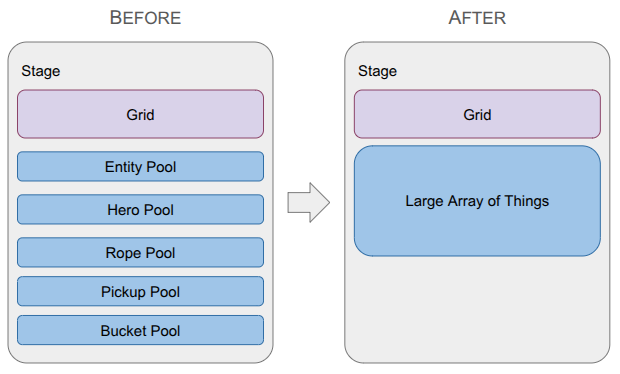
A depiction of the change in the data structure used to represent game entities, going from type-specific lists with a top-level entity table to a single large array of things.

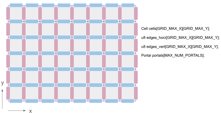
Last month was a big overhaul of the underlying grid representation in order to be able to handle portals. This month ended up being another major refactor, but instead of the grid, I overhauled how game entities are stored.

I wanted to get Pickups back into the game in order to get the fundamental game loop: Heroes enter levels, gather Pickups, and exit to unlock items that make them more powerful. Once Pickups were working, I wanted to add other core mechanics like ropes (for climbing) and buckets (which hold Pickups and can be hoisted via ropes).

All of this logic made it very clear that my current way of interacting with entities was too cumbersome. I had a top-level Entity type that could be looked up by any entity’s ID, and then would itself contain a type enum and a type-specific ID in order to look up the specialized data in the type-specific list. That looked something like:

// Grab the hero.
const Entity* entity = Get(stage.pool_entity, entity_id);
ASSERT(entity != nullptr && entity.type == EntityType::HERO);
Hero* hero = GetMutable(stage.pool_hero, entity.type_id);

After this change, there is no indirection. All entities are in a single array:

// Grab the hero.
const StageThing* thing = Get(stage.things, entity_id);
ASSERT(thing.type == EntityType::HERO);
// Now we can directly access `thing.hero` and do stuff.

Making the transition to a Large Array of Things' data structure removed this annoying indirection. More importantly, it simplified how concepts are shared across entities (e.g., all StageThings now have a cell index). That shared context streamlined my event system - an AttachTo event no longer needs special logic for buckets vs. ropes vs. heroes – and drastically simplified my undo/redo system.

With this new architecture, I was finally able to implement some basic gameplay:

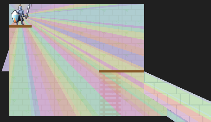
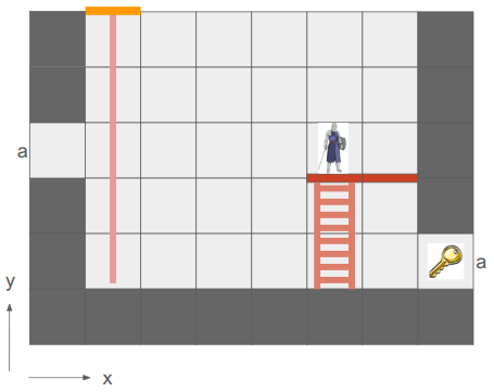
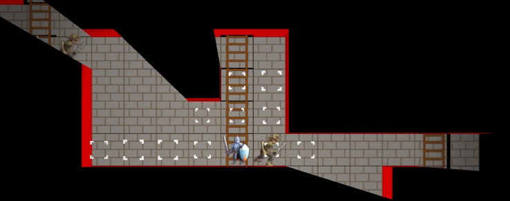
This video shows the state of the game at the time of writing. We see the rope being equipped before entering a basic level. The knight then deploys the rope, which the sorceress can then use to climb down, pick up a relic, and then climb back out. Graphics and UI are very rough first passes.

The rest of this post will cover why I used the original approach, what the Large Array of Things is, and how it led to these improvements.

Old Method: Type-Specific Lists

I started with type-specific lists for every entity type in my game, following what I understood was Billy Basso’s approach on Animal Well. Every entity type gets a struct, and we maintain an array of each struct type that has some max capacity, and we keep the array densely packed as entities are added or removed:

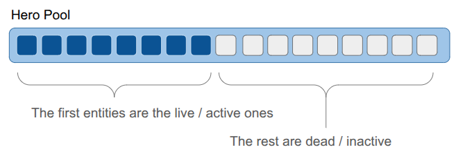
Keeping the live entities packed in the front makes iteration over the entities really fast. We only need to iterate over the first N elements, and they are all sequential in memory.

However, keeping the entities packed means that if an entity is deleted, we will move other entities around:

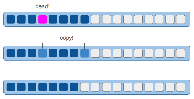
The result is that we can’t reliably point to an entity with a pointer, since its location in memory can change. To solve this, each ObjectPool maintained an extra layer of indirection. Each entity was referred to by an ID, which indexed into a lookup table to find the struct’s actual array index. All of this was managed internally by the pool, so the user never had to track it. I didn’t find this problematic at all.

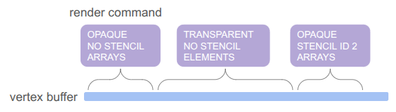
At the beginning of game development, I was iterating through my lists of types quite a lot. Rendering was effectively:

for (hero in heroes) {
    RenderHero(hero)
end
for (rope in ropes) {
    RenderRope(rope)
end
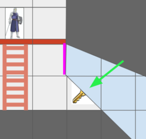
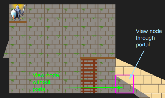
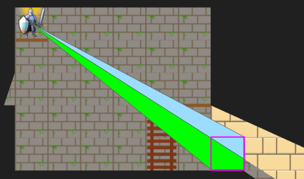
// etc.

That approach was fine before I introduced portals. Now, the same tile might show up in multiple places on the screen. I was no longer able to just loop through the entities to render them; the entities themselves didn’t know where their cells were located in the final view. The iteration had to go the other way:

for (x in view.lo.x to view.hi.x) {
    for (y in view.lo.y to view.hi.y) {
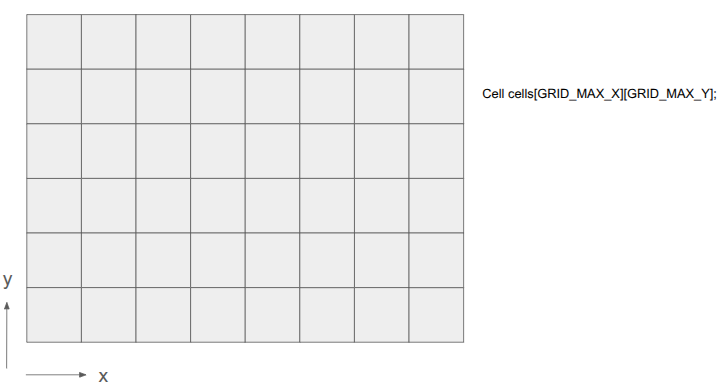
        cell = grid.cells[x][y]
        for (entity in cell) {
            RenderEntityAt(entity, x, y)
        }
    }
}

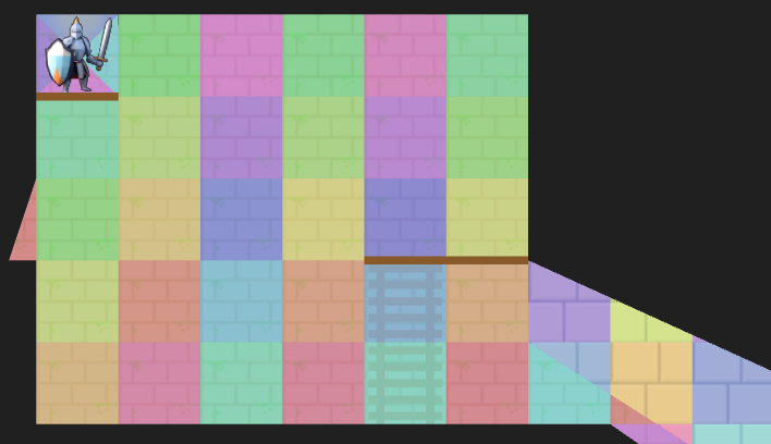
With spatial iteration taking over, the primary benefit of densely packed lists completely disappeared. Yet, I was still paying the cost of indirection—which, honestly, was more about code line-count overhead than runtime performance—every single time I accessed an entity.

Old Method: Top-Level Entity List

The type-specific lists were not sufficient when it came to entities referring to other entities. For example, a rope might refer to the entity holding it. Initially, maybe I knew that would always be a hero, and I could use the hero’s pool index. However, if I later wanted to additionally allow tying a rope to, say, a piton, I’d have to use some cumbersome union. The same issue applied to held objects. A hero might hold a rope, a bucket, or a pickup. If I used a union to store the reference, I would have to update that union—and all the branching logic tied to it—every time I added a new type of holdable item to the game. I needed a more general entity reference.

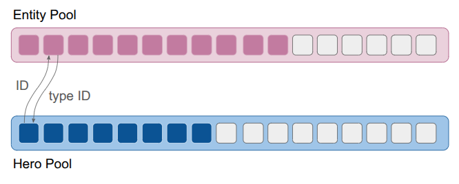
The solution I went with was another list, this time of a generic Entity struct that would contain both the entity’s type enum and its type-specific ID. I also stored additional IDs that let me refer to entities generically, across levels (a feature that was never fully fleshed out). The resulting struct was small, and just enough to support the double-lookup:

struct Entity {
    // The type of entity enum
    EntityType type;
    // The identifier for the entity among all entities in a stage
    EntityId id;
    // The entity's index into the object pool for its type
    EntityId type_id;
    // A globally unique ID for the entity for
    // referring to an entity in the game across all levels.
    // All entities defined for a level have a UID.
    // For other entities (like those spawned temporarily in a stage),
    // this is kInvalidEntityUid.
    EntityUid uid;
};

As discussed earlier, this system required that, given an EntityId, I first look up the Entity struct and then use the entity’s type to identify the type-specific pool and access the type-specific data via the type ID. In addition, actions on entities had to be specialized to each entity type, which made the event system complicated. Finally, I wasn’t taking advantage of the tightly packed object lists, so there wasn’t much keeping me on the current system other than momentum.

Large Array of Things

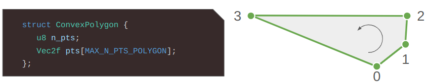
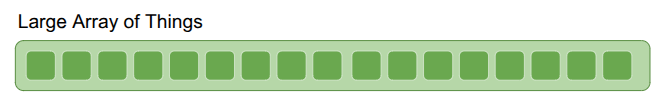
I also learned about the Large Array of Things from the Wookash podcast, in an episode with Anton Mikhailov. This data structure is basically and array of fat structs – rather than having a different collection for every entity type, you define _one_ struct that all entities, or Things, rather, use. The data structure is extremely simple – just an array of Things:

If we want lists, we can hook Things together using intrusive pointers. Any Thing can “point” to another Thing via its integer index. We get a list by maintaining an external index to the head Thing:

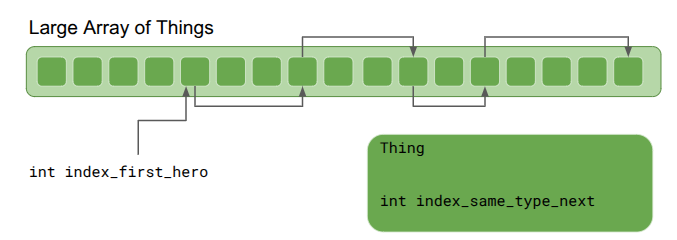
Iteration through the list simply starts with the first Thing and goes until the index is invalid:

int index_next = index_first_hero;
while (index_next != kInvalidThingIndex) {
   Thing& thing = things[index_next];
   DoSomething(thing);
   index_next = thing.index_same_type_next;
}

That works just fine, but we do have to (1) make sure to initialize all things with index_same_type_next = kInvalidThingIndex and (2) if we accidentally use thing.index_same_type_next with a bad index, we could go out-of-bounds. Anton recommended making all such reference lists circular:

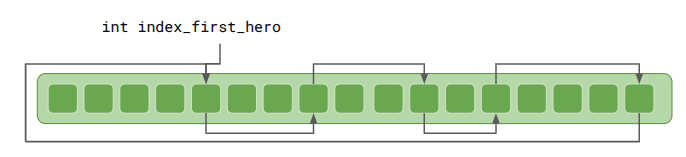
This means thing.index_same_type_next should always be valid. If a Thing is the only one of its type, it will will point to itself.

Iteration is very similar, and has the advantage that one can start from anywhere in the list:

int index_next = index_first_hero;
do {
   Thing& thing = things[index_next];
   DoSomething(thing);
   index_next = thing.index_same_type_next;
} while (index_next != index_first_hero);

In addition to lists, indexing can also be used to represent trees:

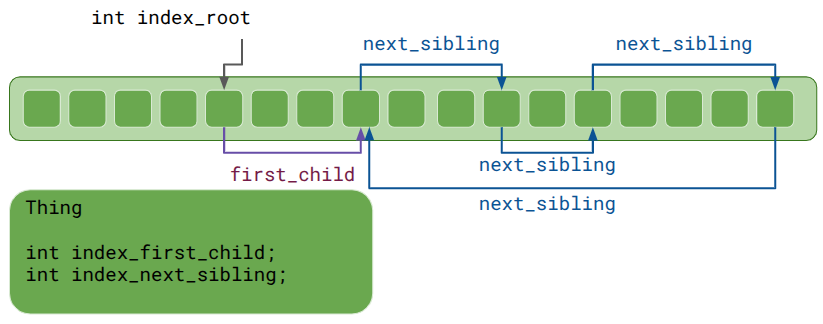
Each Thing has a head index to a list of children, which then reference each other using sibling indices.

It makes less sense here for the head index, index_first_child, to simply point back at the same Thing, since a parent-child relationship is not a circular list. Anton Mikhailov recommended using zero for the invalid index rather than a truly invalid index like -1 in order prevent crashes. Yes, you should never access a Thing at an invalid index, but at least your game doesn’t explode in prod if a rare code path does. Plus, this means zero-initialization defaults those indices to invalid.

As a side effect, the very first Thing is never used. That is a small price to pay, especially if you’re likely going to allocate 10,000.

Lastly, Anton Mikhailov said it is often useful to use doubly-linked lists instead of singly linked lists. This makes insertion and deletion O(1). For trees, it is very useful for a child to know its parent.

So what does a Thing struct look like? Here is my current implementation:

enum class StageThingType : u8 {
    FREE         = 0, // An inactive stage thing
    HERO         = 1, // aka Player Character
    INTERACTABLE = 2,
    ROPE_SEGMENT = 3,
    COUNT        = 4, // Sentinal value
};

// A thing whose state we track in the stage.
// This follows the Large Array of Things approach.
struct StageThing {
    // The type of thing it is.
    StageThingType type;

    // The generational index of the thing in the array of things.
    ThingId id;

    // The index of the next thing of the same type.
    // This is a circular list.
    int index_same_type_next;
    int index_same_type_prev;

    // Which cell in the stage it is in.
    CellIndex cell_index;

    // The index of the next thing in the same cell.
    // This is a circular list.
    int index_same_cell_next;
    int index_same_cell_prev;

    Direction facing_dir;
    // Tree links.
    // Parents and children are always in the same cell index.
    // The sibling list is circular.
    int index_parent;
    int index_first_child;
    int index_next_sibling;
    int index_prev_sibling;

    union {
        StageThingHero hero;
        StageThingInteractable interactable;
        StageThingRopeSegment rope_segment;
    };
};

I went with a union of type-specific structures for now, since it was the most natural conversion of what I was translating from. However, team fat struct may end up convincing me. We’ll see.

We need an additional struct to store the array and the list heads:

struct LargeArrayOfStageThings {
    StageThing things[MAX_NUM_THINGS];
    int count;

    // An array of heads for doubly-linked lists.
    // Index 0 (StageThingType::FREE) is the free list.
    int type_list_heads[(int)StageThingType::COUNT];

    // An array of heads for doubly-linked lists of things in each cell.
    int cell_first_thing[GRID_MAX_X][GRID_MAX_Y];
};

As we can see, the StageThing type zero is for free / inactive Things, letting us use the same list to quickly grab the next available Thing any time we spawn a new one, or stitch it into the list if a Thing is no longer needed. Then there are a bunch of methods that maintain invariants, such as initialization, getting a Thing, attaching a child to a parent, etc.

Indices maintained by the `LargeArrayOfStageThings` itself, such as the linked type list, can be simple integers. Other indices, especially external references, shouldn’t use direct indices since the underlying Thing might be removed in the interim. (This is the same problem as keeping a pointer reference to an Entity.)

The standard mitigation, which I was already employing in my ObjectPools previously, is to use a generational index. Instead of a bare index, it is an index paired with a generation counter:

struct ThingId {
    int index;  // index in the array of things
    u32 gen;    // generation counter
}

Retrieving a Thing via such an ID simply looks at the Thing at the given index, but also checks to make sure the generation counter matches. If it does, we return it. If the Thing has been deleted, or if it has been re-used, the generation counter will have been incremented, and the counter will not match. Since we’re using a u32, there is basically zero risk of wrap around. (Though you can always use u64 if that’s a problem for you.)

Sharing Concepts

Having the shared StageThing struct means we can share concepts across all entity types. The first example is the cell index. Every StageThing can be placed in a cell. This doesn’t mean I have to use it, but so far I am. The direct result is that I can have a single codepath for PlaceInCell, which doesn’t have to have branching logic for heroes vs. ropes vs. enemies, and the LargeArrayOfStageThings can automatically update the internal list of things in each cell.

This drastically simplified my event system. Before this change, the AttachTo event required distinct code paths for every single entity type. Now, attaching is universal for all entities—it is simply a parent/child relationship.

You’ll notice that the StageThingType enum does not contain Pickup or Bucket types. I actually consolidated those into a single type – Interactable. This happened when I started considering how a Pickup could be set down or picked up, but so too could a Bucket. The Bucket simply had additional capabilities, such as allowing other things to be placed in it.

The aha moment here is recognizing that we care about functionalities rather than what a thing is categorically. So, the Interactable has a bitmask that identifies what the thing can do – can it be placed, hung, acquired, used to contain other things, etc? When it comes to the code logic, that is ultimately what it needs to know. Do I or do I not run the logic for this capability?

This is exactly the insight the fat struct folks advocate for. Seeing this simplification, I am seriously tempted to go all-in on the fat struct approach.

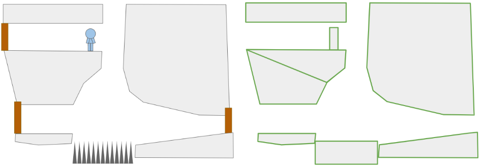
The final part of simplification was now recognizing that all entities are contained in at most a single cell. Prior to this, my rope entity spanned multiple cells. I now have a RopeSegment type instead, which is exactly one cell and has links to the RopeSegment it is connected to above or below. This works really well with the centralized cell lists and handles portals seamlessly.

Here we see a rope being lowered through a portal. The sorceress then climbs down it.

Undo and Redo

I want undo and redo to be supported from the get-go, and to “just work”. Every action must be reversible, and after being reversed, we should be able to re-commit it.

In this post, I covered the event system. Any action builds out a schedule of events that then can be played out. I supported undo and redo by collapsing the schedule into just the set of events needed to get the overall state change needed. For example, if a hero moves three times, which are three cell index change events, I could collapse that into just one cell index change event for undo / redo purposes.

Unfortunately, the logic to do this got rather involved. Any new field that I added to my entities might require a new custom event that I would then have to detect and inject. I also had several “larger” events like hoisting a rope up or down that manifested as a multitude of smaller events. Moving a rope up means adjusting all RopeSegments in the chain. I’d then have to iterate over all of those to see if there were diffs, and figure out the right events to add to the undo / redo sets to get the right result. A big headache.

Instead, I shifted from a delta-based approach to a snapshot approach. I implemented a single, special master event that lets me replace an entire StageThing. That’s it. Now, undo / redo entirely consist of these snapshot events, which overwrite the entire struct (plus the pass turn event – that isn’t in the large array of things). Executing an undo or redo simply applies these state-overwrites and then triggers a rebuild of type_list_heads and cell_first_thing in the LargeArrayOfStageThings. Incredibly simple. Since we’re not undoing and redoing all that often, the cost of that rebuild is insignificant.

Conclusion

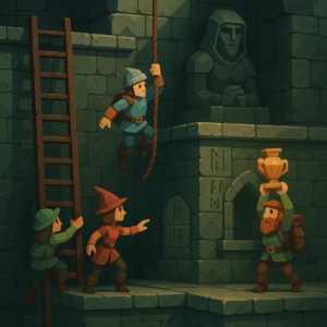
I’m happy to have this entity refactor behind me, but I also feel like it was a great architectural experience and showed how simplicity can compound. This new foundation feels like a good one to build out from. I plan to start expanding on these core mechanics and perhaps touch up some of those rough first-pass graphics. As always, no promises on specifics! We will let the project dictate how it should evolve next.

This post expands on the previous post, which looked at collision detection and resolution for 2d polygons. By the end we were able to apply impulses to colliding bodies to properly get them to bounce and spin off of one another. Not only will we take it further with friction impulses and joints, but we’ll pay special attention to how these impulses are derived to emphasize that this line of reasoning is a tool that can be extended to new applications.

There is more math in this post than normal because I want to both provide a resource that I myself could have benefited from and show that this stuff can all be derived.

An impulse \(\boldsymbol{j}\) is an instantaneous change in momentum. They are very similar to forces, which influence velocity over time:

\[\boldsymbol{f} = m \boldsymbol{a} \quad \Rightarrow \quad \boldsymbol{v}’ \approx \boldsymbol{v} + \frac{1}{m} \boldsymbol{f} \Delta t\]

An impulse applied to a rigid body at a point \(\boldsymbol{r}\) relative to the body’s center of mass similarly affects its velocity, but without the need for the timestep:

\[\boldsymbol{v}’ = \boldsymbol{v} + \frac{1}{m} \boldsymbol{j}\]

This impulse also effects the angular velocity:

\[\boldsymbol{\omega}’ = \boldsymbol{\omega} + \boldsymbol{I}^{-1} \boldsymbol{r} \times \boldsymbol{j}\]

This update models the angular velocity in three dimensions, treating it as a vector. We can work out the equivalent 2d update where we just keep track of a scalar \(\omega\):

\[\begin{align}\boldsymbol{r} \times \boldsymbol{j} = \begin{bmatrix} r_x \\ r_y \\ 0\end{bmatrix}\end{align} \times \begin{bmatrix}j_x \\ j_y \\ 0\end{bmatrix} = \begin{bmatrix} 0 \\ 0 \\ r_x j_y – r_y j_x \end{bmatrix}\]

If we assume our inertia tensor is diagonal, and just pull out the z entry \(I_{zz}\), we get:

\[\omega’ = \omega + \frac{1}{I_{zz}} \left(r_x j_y – r_y j_x\right)\]

From here on out, if you see a scalar \(I\), it refers to \(I_zz\).

The Normal Impulse

In the last blog post, we used an impulse along the impact normal to cause two colliding rigid bodies to bounce off each other. We’re going to cover the same thing, but derive it instead of just take the result for granted.

We have two bodies, A and B, and a contact point located at \(\boldsymbol{r}_A\) relative to body A’s center and at \(\boldsymbol{r}_B\) relative to body B’s center:

The velocity of the contact points on each body as they enter the collision is:

\[\begin{align}\boldsymbol{v}_{cA} & = \boldsymbol{v}_A + \boldsymbol{\omega}_A \times \boldsymbol{r}_A \\ \boldsymbol{v}_{cB} &= \boldsymbol{v}_B + \boldsymbol{\omega}_B \times \boldsymbol{r}_B \end{align}\]

In 2D that amounts to:

\[\boldsymbol{v}_{cA} = \begin{bmatrix}v_{A,x} \\ v_{A,y} \\ 0\end{bmatrix} + \begin{bmatrix}0 \\ 0 \\ \omega_A\end{bmatrix} \times \begin{bmatrix} r_{A,x} \\ r_{A,y} \\ 0\end{bmatrix} = \begin{bmatrix}v_{A,x} \\ v_{A,y} \\ 0\end{bmatrix} + \begin{bmatrix}-\omega r_{A,y} \\ \hphantom{-}\omega r_{A,x} \\ 0\end{bmatrix} \]

One can do this stuff in 3D and then drop or ignore the \(z\)-axis, but in my code I just stick with 2D:

Vec2f r; // radius
Vec2f v; // linear velocity vector
f32 w;   // angular velocity
Vec2f v_c = v + w * Rotr(r);

The contact velocity — how fast the contact points collide — is the relative speed of the contact points:

\[\boldsymbol{v}_\text{rel} = \boldsymbol{v}_{cB} \> – \boldsymbol{v}_{cA}\]

To derive the impulse, we stipulate two things. First, that the impulse lies in the normal direction:

\[\boldsymbol{j} = j \hat{\boldsymbol{n}}\]

Second, that the relative velocity along the normal direction reverses sign and changes by a factor \(e\):

\[\boldsymbol{v}_\text{rel}’ \cdot \hat{\boldsymbol{n}} = \> – e \> \boldsymbol{v}_\text{rel} \cdot \hat{\boldsymbol{n}}\]

This factor \(e\) is called the restitution. Setting it to zero produces a perfectly inelastic collision (because the resulting relative velocity in the normal direction is zero), whereas setting it to 1 produces a perfectly elastic collision that preserves the kinetic energy. Most objects use a value somewhere in-between.

We now have everything we need to derive the impulse. Let’s expand the left-hand side of the restitution equation:

\[\begin{align}\boldsymbol{v}_\text{rel}’ \cdot \hat{\boldsymbol{n}} \\ \left(\boldsymbol{v}_{cB}’ \> – \boldsymbol{v}_{cA}’\right) \cdot \hat{\boldsymbol{n}} \\ \left[\left(\boldsymbol{v}_B’ + \boldsymbol{\omega}_B’ \times \boldsymbol{r}_B\right) – \left(\boldsymbol{v}_A’ + \boldsymbol{\omega}_A’ \times \boldsymbol{r}_A\right)\right] \cdot \hat{\boldsymbol{n}} \\ \left[\left(\left[\boldsymbol{v}_B + \frac{1}{m_B}\boldsymbol{j}\right] + \left[\boldsymbol{\omega}_B + \boldsymbol{I}_B^{-1} \boldsymbol{r}_B \times \boldsymbol{j}\right] \times \boldsymbol{r}_B\right) – \left(\left[\boldsymbol{v}_A – \frac{1}{m_A}\boldsymbol{j}\right] + \left[\boldsymbol{\omega}_A – \boldsymbol{I}_A^{-1} \boldsymbol{r}_A \times \boldsymbol{j}\right] \times \boldsymbol{r}_A\right)\right] \cdot \hat{\boldsymbol{n}} \\ \left[\left(\left[\boldsymbol{v}_B + j \frac{1}{m_B}\hat{\boldsymbol{n}}\right] + \left[\boldsymbol{\omega}_B + j \boldsymbol{I}_B^{-1} \boldsymbol{r}_B \times \hat{\boldsymbol{n}}\right] \times \boldsymbol{r}_B\right) – \left(\left[\boldsymbol{v}_A – j \frac{1}{m_A}\hat{\boldsymbol{n}}\right] + \left[\boldsymbol{\omega}_A – j \boldsymbol{I}_A^{-1} \boldsymbol{r}_A \times \hat{\boldsymbol{n}}\right] \times \boldsymbol{r}_A\right)\right] \cdot \hat{\boldsymbol{n}} \\ \left[\boldsymbol{v}_\text{rel} + j \left(\frac{1}{m_B}\hat{\boldsymbol{n}} + \left[ \boldsymbol{I}_B^{-1} \boldsymbol{r}_B \times \hat{\boldsymbol{n}}\right] \times \boldsymbol{r}_B + \frac{1}{m_A}\hat{\boldsymbol{n}} + \left[ \boldsymbol{I}_A^{-1} \boldsymbol{r}_A \times \hat{\boldsymbol{n}}\right] \times \boldsymbol{r}_A\right)\right] \cdot \hat{\boldsymbol{n}} \\ \boldsymbol{v}_\text{rel} \cdot \hat{\boldsymbol{n}} + j \left(\frac{1}{m_A}\hat{\boldsymbol{n}} + \frac{1}{m_B}\hat{\boldsymbol{n}} + \left[ \boldsymbol{I}_A^{-1} \boldsymbol{r}_A \times \hat{\boldsymbol{n}}\right] \times \boldsymbol{r}_A + \left[ \boldsymbol{I}_B^{-1} \boldsymbol{r}_B \times \hat{\boldsymbol{n}}\right] \times \boldsymbol{r}_B\right) \cdot \hat{\boldsymbol{n}} \\ \boldsymbol{v}_\text{rel} \cdot \hat{\boldsymbol{n}} + j \left(\frac{1}{m_A}\hat{\boldsymbol{n}}\cdot \hat{\boldsymbol{n}} + \frac{1}{m_B}\hat{\boldsymbol{n}}\cdot \hat{\boldsymbol{n}} + \left[ \boldsymbol{I}_A^{-1} \boldsymbol{r}_A \times \hat{\boldsymbol{n}}\right] \times \boldsymbol{r}_A \cdot \hat{\boldsymbol{n}} + \left[ \boldsymbol{I}_B^{-1} \boldsymbol{r}_B \times \hat{\boldsymbol{n}}\right] \times \boldsymbol{r}_B \cdot \hat{\boldsymbol{n}}\right) \\ \boldsymbol{v}_\text{rel} \cdot \hat{\boldsymbol{n}} + j \left(\frac{1}{m_A} + \frac{1}{m_B} + \left[ \boldsymbol{I}_A^{-1} \boldsymbol{r}_A \times \hat{\boldsymbol{n}}\right] \times \boldsymbol{r}_A \cdot \hat{\boldsymbol{n}} + \left[ \boldsymbol{I}_B^{-1} \boldsymbol{r}_B \times \hat{\boldsymbol{n}}\right] \times \boldsymbol{r}_B \cdot \hat{\boldsymbol{n}}\right) \end{align}\]

We then equate this to \( – e \> \boldsymbol{v}_\text{rel} \cdot \hat{\boldsymbol{n}}\) and solve for the impulse scalar \(j\), yielding:

\[j = \frac{-(1+e) \boldsymbol{v}_\text{rel} \cdot \hat{\boldsymbol{n}} }{ \frac{1}{m_A} + \frac{1}{m_B} + \left(\left[ \boldsymbol{I}_A^{-1} \boldsymbol{r}_A \times \hat{\boldsymbol{n}}\right] \times \boldsymbol{r}_A + \left[ \boldsymbol{I}_B^{-1} \boldsymbol{r}_B \times \hat{\boldsymbol{n}}\right] \times \boldsymbol{r}_B\right) \cdot \hat{\boldsymbol{n}} }\]

This is the equation that Wikipedia gives us.

The equation I gave in the last blog post looks a little different:

\[j = \frac{-(1+e)\boldsymbol{v}_\text{rel} \cdot \hat{\boldsymbol{n}}}{\frac{1}{m_A} + \frac{1}{m_B} + \frac{(\boldsymbol{r}_A \times \boldsymbol{n})^2}{I_A} + \frac{(\boldsymbol{r}_B \times \boldsymbol{n})^2}{I_B}}\]

It only differs in the terms involving the moment of inertia.

Let’s expand the Wikipedia version:

\[\begin{align}\left[\left(\boldsymbol{I}^{-1} \boldsymbol{r} \times \hat{\boldsymbol{n}}\right) \times \boldsymbol{r}\right] \cdot \hat{\boldsymbol{n}} &= \left(\left(\frac{1}{I}\begin{bmatrix}r_x \\ r_y \\ 0\end{bmatrix} \times \begin{bmatrix} \hat{n}_x \\ \hat{n}_y \\ 0 \end{bmatrix}\right) \times \begin{bmatrix}r_x \\ r_y \\ 0\end{bmatrix}\right) \cdot \begin{bmatrix}\hat{n}_x \\ \hat{n}_y \\ 0\end{bmatrix} \\ &= \left(\frac{1}{I}\begin{bmatrix}0 \\ 0 \\ r_x \hat{n}_y – r_y \hat{n}_x\end{bmatrix} \times \begin{bmatrix}r_x \\ r_y \\ 0\end{bmatrix}\right) \cdot \begin{bmatrix}\hat{n}_x \\ \hat{n}_y \\ 0\end{bmatrix} \\ &= \frac{1}{I}\begin{bmatrix}-r_x r_y \hat{n}_y + r_y^2 \hat{n}_x \\ r_x^2 \hat{n}_y – r_x r_y \hat{n}_x \\ 0 \end{bmatrix} \cdot \begin{bmatrix}\hat{n}_x \\ \hat{n}_y \\ 0\end{bmatrix} \\ &= \frac{1}{I}\left( r_x^2 \hat{u}_y^2 – 2 r_x r_y \hat{u}_x \hat{u}_y + r_y^2 \hat{u}_y^2 \right) \end{align}\]

We get the same thing if we expand the other version:

\[\begin{align}\frac{1}{I}\left(\boldsymbol{r} \times \hat{\boldsymbol{n}}\right)^2 &= \frac{1}{I}\left(r_x \hat{n}_y – r_y \hat{n}_x\right)^2 \\ &= \frac{1}{I}\left( r_x^2 \hat{u}_y^2 – 2 r_x r_y \hat{u}_x \hat{u}_y + r_y^2 \hat{u}_y^2 \right)\end{align}\]

The two formulations are equal, but assume that we’re working in 2D and that the moment of inertia tensor is diagonal with every entry equal to \(I\). The Wikipedia version is more general, and can handle 3D collisions and general inertia tensors.

The normal impulse \(j\) in 2D is thus

\[j = \> -(1+e) \> m_\text{eff} \> \boldsymbol{v}_\text{rel} \cdot \hat{\boldsymbol{n}} \]

where the effective mass is

\[m_\text{eff} = \left(\frac{1}{m_A} + \frac{1}{m_B} + \frac{(\boldsymbol{r}_A \times \hat{\boldsymbol{n}})^2}{I_A} + \frac{(\boldsymbol{r}_B \times \hat{\boldsymbol{n}})^2}{I_B}\right)^{-1}\]

After calculating it, we apply an impulse \(j \hat{\boldsymbol{n}}\) to body B and the negated impulse to body A. Note that we only apply an impulse if the relative velocity is causing the bodies to move into contact (\(\boldsymbol{v}_\text{rel} \cdot \hat{\boldsymbol{n}} < 0\)), otherwise the contact point already has a separating velocity.

The restitution \(e\) will depend on the colliding bodies. One convenient way to get it is to assign an restitution to each rigid body, and then use the maximum between the two for the collision. That allows bounciness to win out:

\[e = \max\left(e_A, e_B\right)\]

Friction Impulse

The normal impulse takes care of the relative penetration speed, but does nothing in the tangent direction along the contact line. We typically want shapes that slide along each other to have friction — that is what the friction impulse, or tangent impulse, is for.

Wikipedia and other websites will at this point show you a fancy diagram for Coulomb friction depicting the friction cone. I don’t find that to be particularly illuminating.

Instead, I simply like to think about Coulomb friction as:

• compute a tangent impulse that causes the relative tangent velocity to be zero (\(e=0\))
• if the required tangent impulse is sufficiently small, apply it (static friction)
• if the required tangent impulse is too large, cap it out and apply that instead (dynamic friction)

Let’s derive the update ourselves again.

The friction impulse acts in the tangent direction \(\hat{\boldsymbol{t}}\), which we can get by rotating the normal. We once again have a scalar impulse:

\[j = j \hat{\boldsymbol{t}}\]

We compute the tangent that causes a zero relative tangent velocity (\(e = 0\)).

These two conditions are structurally the same as the normal impulse, except \(e\) is fixed. We can directly apply our previous equations to get:

\[j = \> – m_\text{eff} \> \boldsymbol{v}_\text{rel} \cdot \hat{\boldsymbol{t}}\]

where the effective mass is now in the tangent direction:

\[m_\text{eff} = \left(\frac{1}{m_A} + \frac{1}{m_B} + \frac{(\boldsymbol{r}_A \times \hat{\boldsymbol{t}})^2}{I_A} + \frac{(\boldsymbol{r}_B \times \hat{\boldsymbol{t}})^2}{I_B}\right)^{-1}\]

As long as this impulse is small enough (in magnitude), we apply it in order to prevent any tangential sliding. If it is large enough, we switch from static friction to dynamic friction:

\[j = \begin{cases} j & \text{if } |j| \leq j_\text{static} \\ j_\text{dynamic} & \text{otherwise} \end{cases}\]

Easy peasy.

The static and dynamic friction values are typically multiples of the normal impulse. We multiply the normal impulse by \(\mu_\text{static}\) to get the static friction impulse threshold and by \(\mu_\text{dynamic}\) to get the dynamic friction impulse threshold. Like the restitution, these are properties of each body, and we can obtain values to use for a pair of bodies by combining their values. Here it is recommended to use the square root of the product, which lets extremely low-friction (slippery) values dominate:

\[\mu_\text{static} = \sqrt{\vphantom{P}\mu_{A,\text{static}} \cdot \mu_{B,\text{static}}}\]

Revolute Joints

There are other things we can do with impulses. One of the main ones is to model attachment points between rigid bodies. These revolute joints allow rotation, but force the bodies to maintain a constant distance vector to the joint:

Revolute joints are useful for all sorts of things, including swinging:

I didn’t have a lot of luck finding information on how to enforce revolute joints between rigid bodies in 2D. Thankfully, we can derive the necessary impulse ourselves.

The property we want to enforce is that the contact velocity at the joint after the impulse be zero:

\[\boldsymbol{v}_\text{rel}’ = \boldsymbol{0}\]

We can expand that out:

\[\begin{align}\boldsymbol{v}_\text{rel}’ &= \boldsymbol{0} \\ \boldsymbol{v}_{cB}’ \> – \boldsymbol{v}_{cA}’ &= \boldsymbol{0} \\ \left(\boldsymbol{v}_B’ + \boldsymbol{\omega}_B’ \times \boldsymbol{r}_B\right) – \left(\boldsymbol{v}_A’ + \boldsymbol{\omega}_A’ \times \boldsymbol{r}_A\right) &= \boldsymbol{0} \\ \left(\left[\boldsymbol{v}_B + \frac{1}{m_B}\boldsymbol{j}\right] + \left[\boldsymbol{\omega}_B + \boldsymbol{I}_B^{-1} \boldsymbol{r}_B \times \boldsymbol{j}\right] \times \boldsymbol{r}_B\right) – \left(\left[\boldsymbol{v}_A – \frac{1}{m_A}\boldsymbol{j}\right] + \left[\boldsymbol{\omega}_A – \boldsymbol{I}_A^{-1} \boldsymbol{r}_A \times \boldsymbol{j}\right] \times \boldsymbol{r}_A\right) &= \boldsymbol{0} \\ \boldsymbol{v}_\text{rel} + \left(\frac{1}{m_B}\boldsymbol{j} + \left[\boldsymbol{I}_B^{-1} \boldsymbol{r}_B \times \boldsymbol{j}\right] \times \boldsymbol{r}_B\right) + \left(\frac{1}{m_A}\boldsymbol{j} + \left[\boldsymbol{I}_A^{-1} \boldsymbol{r}_A \times \boldsymbol{j}\right] \times \boldsymbol{r}_A\right) &= \boldsymbol{0} \\ \boldsymbol{v}_\text{rel} + \left(\frac{1}{m_A} + \frac{1}{m_B}\right)\boldsymbol{j} + \left(\boldsymbol{I}_A^{-1} \boldsymbol{r}_A \times \boldsymbol{j}\right) \times \boldsymbol{r}_A + \left(\boldsymbol{I}_B^{-1} \boldsymbol{r}_B \times \boldsymbol{j}\right) \times \boldsymbol{r}_B &= \boldsymbol{0}\end{align}\]

If we work out the cross products, then we end up with the following system of equations:

\[\begin{bmatrix}\frac{1}{m_A} + \frac{1}{m_B} + \frac{1}{I_A}r_{Ay}^2 + \frac{1}{I_B}r_{By}^2 & -\left(\frac{1}{I_A}r_{Ax}r_{Ay} + \frac{1}{I_B}r_{Bx}r_{By}\right) \\ -\left(\frac{1}{I_A}r_{Ax}r_{Ay} + \frac{1}{I_B}r_{Bx}r_{By}\right) & \frac{1}{m_A} + \frac{1}{m_B} + \frac{1}{I_A}r_{Ax}^2 + \frac{1}{I_B}r_{Bx}^2\end{bmatrix}\begin{bmatrix} j_x \\ j_y\end{bmatrix} = \begin{bmatrix}-v_{\text{rel},x} \\ -v_{\text{rel},y}\end{bmatrix}\]

We can write a simple function that can solve such a \(2 \times 2\) linear system:

// Solve a 2x2 system of linear equations
// [a b][x1] = [e]
// [c d][x2] = [f]
// This method assumes that it will succeed, which
// requires that the matrix be invertible.
template <typename T>
void Solve(T a, T b, T c, T d, T e, T f, T& x1, T& x2) {
    T det = d * a - c * b;
    x2 = (a * f - c * e) / det;
    x1 = (e - b * x2) / a;
}

and then use that to solve for our impulse.

// Compute the effective mass components.
f32 m_eff_11 = inv_m1 + inv_m2 + inv_I1 * r1.y * r1.y + inv_I2 * r2.y * r2.y;
f32 m_eff_12 = -(inv_I1 * r1.x * r1.y + inv_I2 * r2.x * r2.y);
f32 m_eff_22 = inv_m1 + inv_m2 + inv_I1 * r1.x * r1.x + inv_I2 * r2.x * r2.x;

// Solve for the impulse:
//  [m_eff_11   m_eff_12][j.x] = [-v_rel.x]
//  [m_eff_12   m_eff_22][j.y] = [-v_rel.y]
Vec2f j;
Solve(m_eff_11, m_eff_12, m_eff_12, m_eff_22, -v_rel.x, -v_rel.y, j.x, j.y);

We can then apply the resulting impulse to both bodies and perform a positional correction. I weight the correction such that the target joint location is biased toward the heavier object (that way joints on infinite-mass objects never move).

Conclusion

This post set the mathematical foundation for impulses, then derived the normal, friction, and revolute joint impulses. In each case, we looked at what was being preserved, formulated that mathematically, and massaged the equations to back out the impulse. While the equations were long at times, they did not lead us astray and we were able to find our way to some solid physics.