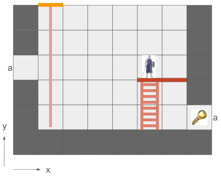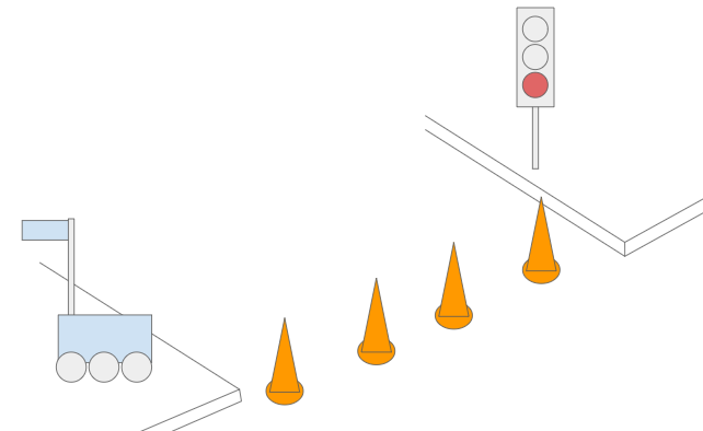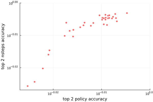
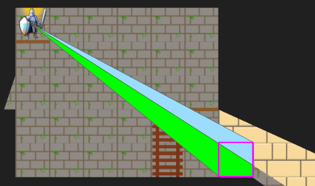
A debug view showing shadow cast segments from the vantage point of the actor.
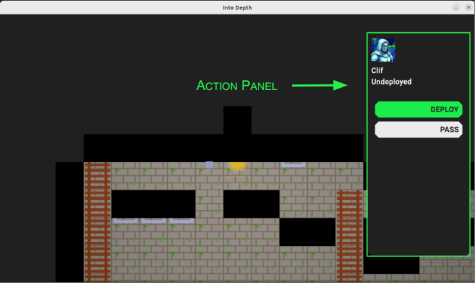
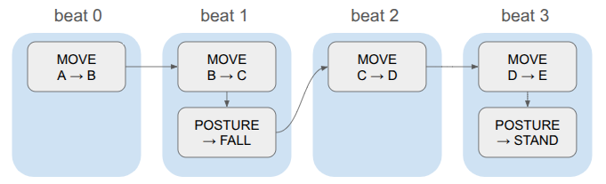
Last month we covered the unified action system, in which we built some basic things players can do with their heroes, and set the stage for fancier futures and actions for enemy agents. The most significant action was moving, which was built based on a GridView of what the actor sees from their current vantage point. As noted in that post, we eventually wanted to expand the grid view to include edge information, such as thin little walls and platforms, but also portals that act as non-Euclidean connections to other parts of the map.
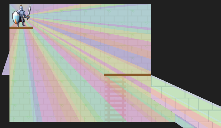
Here we have a simple two-tile room with a loop-back portal on either end. The result – the hero can see a bunch of versions of themselves!
In the last post, I said I’d be adding other entities in and adding more actions, but I decided that the map representation was so fundamental that prioritizing getting these portals in was more important. Any changes there would affect most other systems, so I wanted to get that done first.
Grid Representation
Prior to this change, the underlying level geometry representation, the Grid, was just a 2D array of cells:
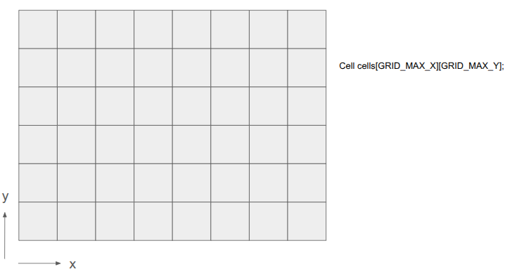
After this change, I wanted to represent both the cells as well as the edges between them:
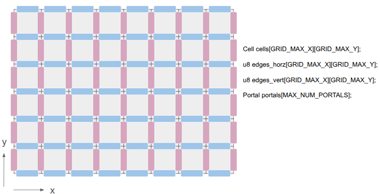
This was achieved by adding two additional 2D arrays, one for the horizontal edges and one for the vertical edges. There are definitely other ways to do this, but I felt that (1) this was simple, and (2) there are differences between those edge types. A player might stand on a platform but have a door that they can open, for example.
The edges are single-bit entries, to keep things efficient. If we need more information, we can index into a separate array. I’m currently using the first two bits to identify the edge type, and the remaining 6 bits, if the edge is a portal, index into a Portal array. The Portal stores the information necessary to know which two edges it links.
This change has the immediate consequence that getting the cell neighbor in a given direction does not necessarily produce the Euclidean neighbor. Its second consequence is that cells no longer need to be solid or not — the edges between cells can instead be solid. This slightly simplifies cells.
Grid View Representation
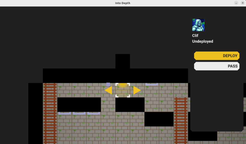
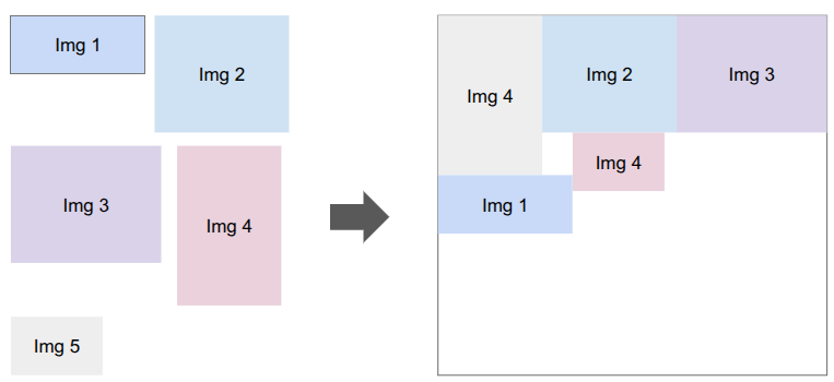
The Grid View, introduced in the last post to represent the level geometry as seen by an actor from their vantage point, can now represent views where the same underlying cell might show up multiple times due to portal connections. Furthermore, we might have weird cases where one square cell might contain slices from different areas of the map:
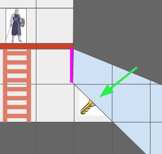
The green arrow points at a view cell which, due to the portal (magenta), has two sections of different grid cells.
Before, the grid view was a simple 2D array with one cell per tile. Now, that is no longer the case.
The updated grid view is organized around ViewNodes, ShadowSegments, and ViewTransforms:
struct GridView {
    // The grid tile the view is centered on
    CellIndex center;

    // The first ViewNode in each view cell.
    // 0xFFFF if there is no view node in that cell.
    u16 head_node_indices[GRID_VIEW_MAX_X][GRID_VIEW_MAX_Y];

    u16 n_nodes;
    ViewNode nodes[GRID_VIEW_MAX_NODES];

    // Shadowcast sectors.
    u16 n_shadow_segments;
    ShadowSegment shadow_segments[GRID_VIEW_MAX_NODES];

    // The transforms for the view as affected by portals.
    u8 n_view_transforms;
    ViewTransform view_transforms[GRID_VIEW_MAX_TRANSFORMS];
};
Most of the time, a given cell in the grid view will contain a single cell in the underlying grid. However, as we saw above, it might see more than one. Thus, we can look up a linked list of ViewNodes per view cell, with an intrusive index to its child (if any). Each such node knows which underlying grid cell it sees, whether it is connected in each cardinal direction to its neighbor view cells, and what sector of the view it contains:
struct ViewNode {
CellIndex cell_index;
// Intrusive data pointer, indexing into the GridView nodes array,
// to the next view node at the same ViewIndex, if any.
// 0xFFFF if there is no next view node.
u16 next_node_index;
// Whether this view node is continuous with the view node in the
// given direction.
// See direction flags.
u8 connections;
// The sector this view node represents.
Sector sector;
// The stencil id for this view node.
// Identical to the transform_index + 1.
u8 stencil_id;
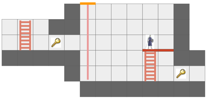
};We can now represent cases like the motivating portal scenario:
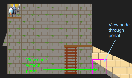
I’ve given the region on the other side of the portal different tile backgrounds to make it more obvious.
In the last post, we constructed the grid view with breadth-first search (BFS) from the center tile. Now, since we’re working with polar segments that strictly expand outwards, we can actually get away with the even simpler depth-first search (DFS). Everything is radial, and the farther out we get, the narrower our beams are:

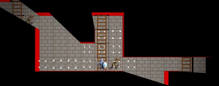
A debug view showing the final shadow cast segments.
The search logic is a bit more complicated given that we have to narrow down the segment every time we pass through a tile’s edge, we’re saving view nodes in the new intrusive linked list structure, and edge traversals have to check for portals. Solid edges terminate and trigger the saving of a shadow segment.
Portal traversals have the added complexity of changing physically where we are in the underlying grid. If we think of the underlying grid as one big mesh, we effectively have to position the mesh differently when rendering the stuff on the other side of the portal. That information is stored in the ViewTransform, and it is also given its own stencil id.
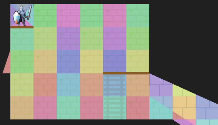
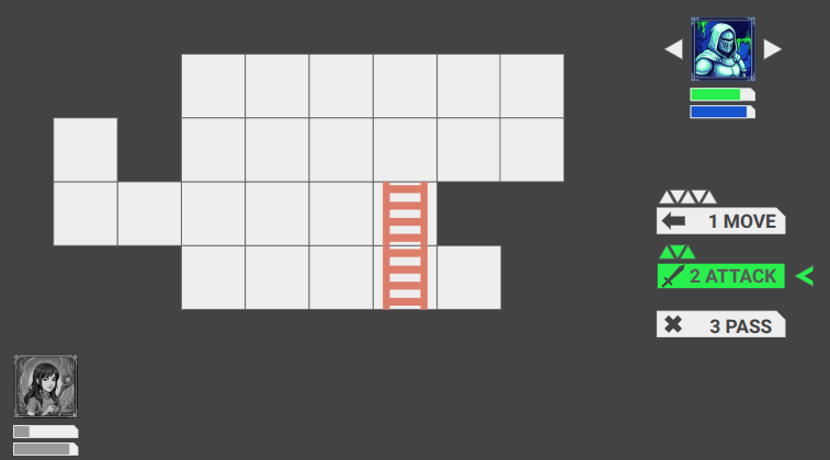
A debug view of the view nodes. We fully see many cells, but some cells we only partially see. The origin is currently split into four views in order for view segments to never exceed 180 degrees.
Above we can see an overlay of the resulting view nodes. There is a little sliver of a cell we can see for a passage off to the left, and there are the two passages, one with a portal, that we can see on the right. The platforms (little brown rectangles) do not block line of sight.
The Stencil Buffer
Now that we have the grid view, how do we render it? It is pretty easy to render a square cell, but do we now have to calculate the part of each cell that intersects with the view segment? We very much want to avoid that!
Clean rendering is accomplished via the stencil buffer, which is a feature in graphics programming that lets us mask out arbitrary parts of the screen when rendering:
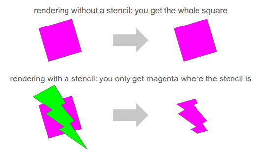
We’ve already been using several buffers when rendering. We’re writing to the RGB color buffers, and 3D occlusion is handled via the depth buffer. The stencil buffer is just an additional buffer (here, one byte per pixel), that we can use to get a stenciling effect.
At one byte (8 bits) per pixel, the stencil buffer can at first glance only hold 8 overlapping stencil masks at once. However, with our 2D orthographic setup, our stencil masks never overlap. So, we can just write 255 unique values per pixel (reserving 0 for the clear).
We simply write the shadow segments to the stencil buffer, setting the buffer to the appropriate stencil ID:
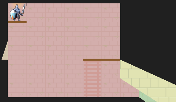
The stencil buffer has four stencil masks – the red region in the main chamber, the little slice of hallway to the left, the green region through the portal leading back into the same room, and the yellow region through a different portal to an entirely different room.
Our rendering pipeline now needs to support masking with these stencil IDs. In January we covered the render setup, which involved six different types of render commands that the game could send to the backend:
- render mesh – render a 3D mesh with lighting, already uploaded to the GPU
- render local mesh – render a 3D mesh without lighting, sending vertices from the CPU
- render quad – an old simple command to render a quad
- render sprite – self-explanatory
- render spritesheet sprite – an old version of render sprite
- render panel – renders a panel with 9-slice scaling by sending vertices from the CPU
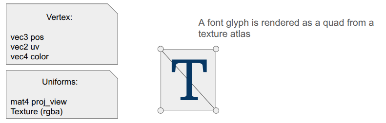
- render text – renders font glyphs by sending quads from the CPU
Having three versions of everything – rendering without stencils, rendering with stencils, and rendering to the stencil buffer itself, would triple the number of command types. That is too much!
Furthermore, we want to order the render commands such that opaque things are drawn front to back, and transparent things are then drawn back to front, and finally drawing UI elements in order at the end. That would require sorting across command types, which seems really messy.
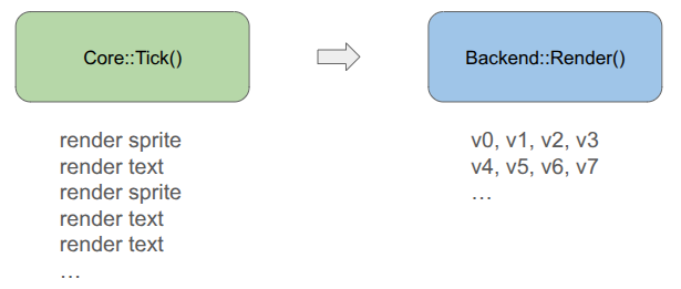
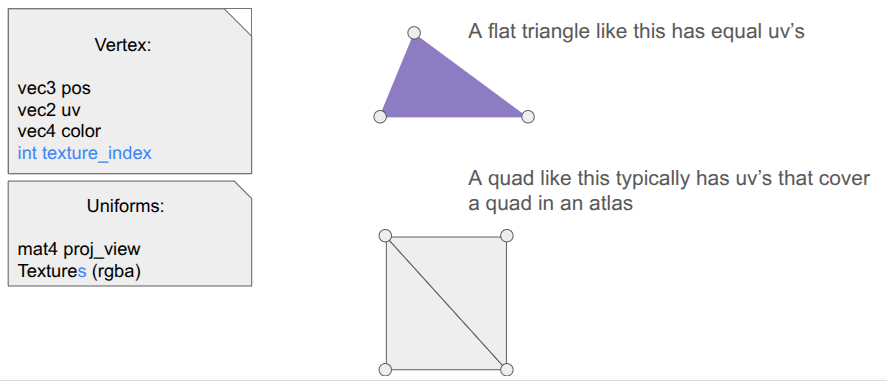
To achieve this all neatly, I collapsed everything sending vertices from the CPU to a unified command type, and have the backend fill the vertex buffer when the game creates the command:
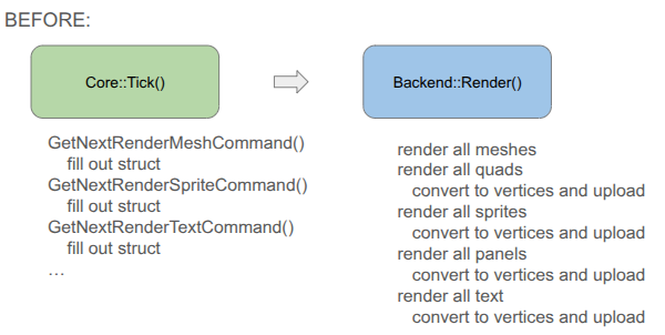
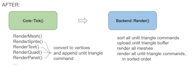
You will notice that the game-side changed a bit. Rather than receiving a command struct and being responsible for populating all fields, I decided to move rendering to methods that expect everything you need to be passed in. This is less error prone, allows for different function signatures that populate what you need, and means I don’t actually need structs for the different command types if we’re directly converting to vertices.
Each unified command (everything but the mesh render calls) is simply:
// Determines the order in which things are rendered.
enum class PassType : u8 {
OPAQUE = 0,
TRANSLUCENT = 1,
UI = 2,
};
// Determines whether and how a command uses a stencil.
enum class StencilRequirement : u8 {
NONE = 0, // Does not use stencils
WRITE = 1, // Writes to the stencil buffer
READ = 2, // Reads from the stencil buffer
};
// Determines how the draw gets executed.
enum class DrawMode : u8 {
ARRAYS, // No EBO
ELEMENTS, // With EB
};
struct RenderCommandUnlitTriangle {
// The commands are sorted by the sort key prior to rendering, determining the order.
// Bits 63-62 (2 bits): Pass Type (Opaque, Translucent, UI)
// Bits 61-60 (2 bits): Stencil Requirement
// Bits 59 (1 bit): Draw Mode
// Bits 58-51 (8 bits): Stencil ID (0 for none)
// Bits 50-32 <reserved>
// Bits 31-0 (32 bits)
// In Opaque: front-to-back distance
// In Translucent: back-to-front distance
// In UI: sequence ID
u64 sort_key;
// Draw Arguments
u32 n_vertices; // Number of vertices to draw
u32 i_vertex; // Index of the start vertex
u32 n_indices; // Number of indices, if using ELEMENTS
u32 i_index; // Index of the start element index, if using ELEMENTS
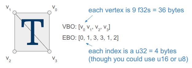
};Apparently, this is much closer to how modern game engines structure their render commands. There is one vertex buffer that we write into as commands are added by the game, and the command just keeps track of the appropriate range. The same is true for the index buffer, which in our case is pre-populated buffer for quad rendering (so each quad takes 4 vertices and 6 indices instead of 6 vertices):
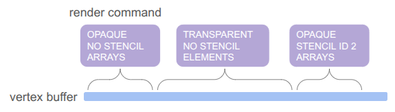
The pass type, stencil requirement, and draw mode are then baked into a sort key that we can sort on in order to automagically get the commands in the order we want: opaque < transparent < UI, with no stencil < write to stencil < read from stencil, and then grouping by whether we use the elements (index) buffer or not. We even use the lower 32 bits for additional sorting, rendering opaque things front to back (since lighting is expensive and we can discard more pixels that way), rendering transparent things back to front (required to get correct results), and rendering UI elements in the order they are created.
Being able to call glBufferData once to send all of the vertices up once at the beginning is really nice. Before, we were writing vertices and sending just the few we needed for every command type each time.
The end result is significantly simpler backend rendering code. It can become even simpler if we eventually unify the mesh rendering with the unlit triangle rendering, but I’m holding off on that because those render commands have a bunch of uniform data and then I’m switching between shaders. I’m not currently rendering transparent meshes, and if I eventually do I’ll bite the bullet and further consolidate.
Conclusion
I am quite happy to have tackled the fundamental grid representation, which as we saw ended up affecting a lot of stuff. The new grid view now needs to be properly integrated into the movement action, and then we can actually start introducing other entities like ropes, buckets and relics. No promises on specifics! We’ll let the project dictate how it should evolve.