Let’s work through how one might (in a broad sense) write a controller for guiding rockets under propulsive control for a pinpoint landing. Such a “planetary soft landing” is central to landing exploratory rovers and some modern rockets. It is also quite an interesting optimization problem, one that starts off seemingly hairy but turns out to be completely doable. There is something incredible about landing rockets, and there is something awesome and inspiring about the way this math problem lets us do just that.
Everything in this post is based off of Lars Blackmore’s paper, Lossless Convexification of Nonconvex Control Bound and Pointing Constraints of the Soft Landing Optimal Control Problem.
Problem Setup
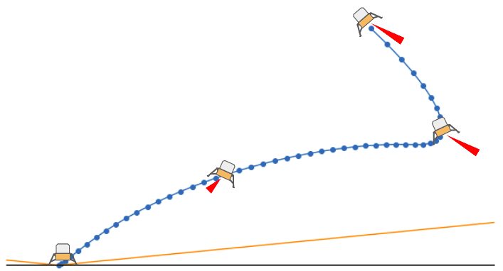
We have a rocket. Our rocket is falling fast, and we wish to have it stop nice and gently on the surface of our planet. We will get it to stop gently by having the rocket use its thruster (or thrusters) to both slow itself down and navigate to a desired landing location.
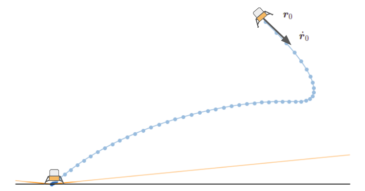
As such, our problem is to find a thrust control profile \(\boldsymbol{T}_c\) to produce a trajectory from an initial position \(\boldsymbol{r}_0\) and initial velocity \(\dot{\boldsymbol{r}}_0\) to a final position at the landing pad with zero final velocity. As multiple trajectories may be feasible, we’ll choose the one that minimizes our fuel use.
We model the rocket as a point-mass. This is done both because it is a lot easier, but also because rockets are pretty stable and we want to maintain a vertical orientation, and any attitude control that we would need has much faster-acting dynamics that we could control separately.
Dynamics
Our state at a given point in time is given by both the physical state \(\boldsymbol{x} = [\boldsymbol{r}, \dot{\boldsymbol{r}}]\) consisting of the position and the velocity, and the rocket’s mass \(m\). I am going to do the derivation in 2D, but it is trivial to extend all of this to the 3D case.
Our physical system dynamics are:
\[\dot{\boldsymbol{x}}(t) = \boldsymbol{A} \boldsymbol{x}(t) + \boldsymbol{B} \left(\boldsymbol{g} + \frac{\boldsymbol{T}_c(t)}{m(t)}\right)\]
where \(\boldsymbol{g}\) is the gravity vector and our matrices are:
\[\boldsymbol{A} = \begin{bmatrix} \boldsymbol{0} & \boldsymbol{I} \\ \boldsymbol{0} & \boldsymbol{0} \end{bmatrix} \qquad \boldsymbol{B} = \begin{bmatrix} \boldsymbol{0} & \boldsymbol{0} \\ \boldsymbol{I} & \boldsymbol{0} \end{bmatrix}\]
for input vectors \([\boldsymbol{r}, \dot{\boldsymbol{r}}]\).
Our mass dynamics are \(\dot{m} = -\alpha \|\boldsymbol{T}_c(t)\|\), where the mass simply decreases in proportion to the thrust. Here \(\alpha\) is the constant thrust-specific fuel consumption that determines our rate of mass loss per unit of thrust.
, such that \(t\) runs from zero to \(t_f\).
Adding Constraints
We can take these dynamics and construct an optimization problem that finds a thrust control profile that brings us from our initial state to our final state with the minimum amount of fuel use. There are, however, a few additional constraints that we need to add.
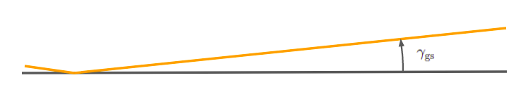
First, we do not want our rocket to go below ground. The way this was handled in the paper was by adding a simple glide-slope constraint that prevents the rocket’s position from ever leaving a cone above the landing location. This ensure that we remain a safe distance above the ground. In 2D this is:
\[r_y(t) \geq \tan(\gamma_\text{gs}) r_x(t) \quad \text{for all } t\]
where \(r_x(t)\) and \(r_y(t)\) are our horizontal and vertical positions at time \(t\), and \(\gamma_\text{gs} \in [0,\pi/2]\) is a glide slope angle.
Next, we need to ensure that we do not use more fuel than what we have available. Let \(m_\text{wet}\) be our wet mass (initial rocket mass, consisting of the rocket plus all fuel), and \(m_\text{dry}\) be our dry mass (just the mass of the rocket – no fuel). Then we need our mass to remain above \(m_\text{dry}\).
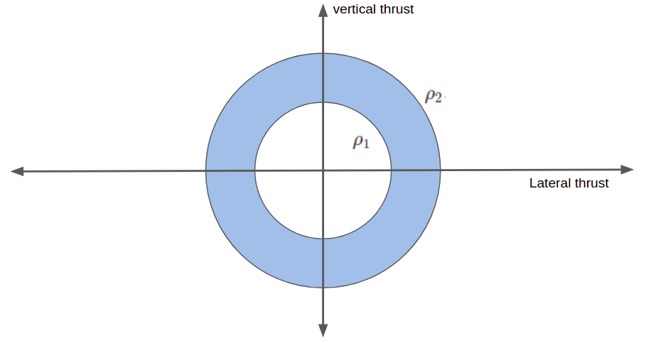
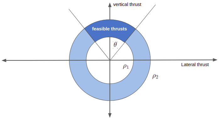
Finally, we have some constraints with respect to our feasible thrust. First off, we cannot produce more thrust than our engine provides: \(\|\boldsymbol{T}_c\| \leq \rho_2\). Secondarily, we also cannot produce less thrust than a certain minimum: \(0 < \rho_1 \leq \|\boldsymbol{T}_c\|\). This lowerbound is caused by many rocket engines being physically unable to reduce thrust to zero without going out. Unfortunately, it is a non-convex constraint, and we will have to work around it later.
The last thrust constraint has to do with how far we can actuate our rocket engines. We are keeping our rocket vertically aligned during landing, and often have a limited ability to gimbal the engine. We introduce a thrust-pointing constraint that limits our deviation from vertical to within an angle \(\theta\):
\[ \boldsymbol{T}_{c,y}(t) \geq \|\boldsymbol{T}_c(t)\| \cos(\theta) \]
Our basic nonconvex minimum fuel landing problem is thus:
\[\begin{matrix}\text{minimize}_{\boldsymbol{T}_c} & \int_0^{t_f} \alpha \|\boldsymbol{T}_c(t)\| \> dt & & \\ \text{subject to} & \dot{\boldsymbol{x}}(t) = \boldsymbol{A} \boldsymbol{x}(t) + \boldsymbol{B} \left(\boldsymbol{g} + \frac{\boldsymbol{T}_c(t)}{m(t)}\right) & \text{for all } t \in [0, t_f] & \text{physical dynamics} \\ & \dot{m} = -\alpha \|\boldsymbol{T}_c(t)\| & \text{for all } t \in [0, t_f] & \text{mass dynamics} \\ & 0 < \rho_1 \leq \|\boldsymbol{T}_c\| \leq \rho_2 & \text{for all } t \in [0, t_f] & \text{thrust magnitude bounds} \\ & \boldsymbol{T}_{c,y}(t) \geq \|\boldsymbol{T}_c(t)\| \cos(\theta) & \text{for all } t \in [0, t_f] & \text{thrust pointing constraint} \\ & r_y(t) \geq \tan(\gamma_\text{gs}) r_x(t)& \text{for all } t \in [0, t_f] & \text{glide slope constraint} \\ & \boldsymbol{r}(0) = \boldsymbol{r}_0, \dot{\boldsymbol{r}}(0) = \dot{\boldsymbol{r}}_0 & & \text{physical initial conditions} \\ & m(0) = m_\text{wet} & & \text{mass initial condition} \\ & \boldsymbol{r}(t_f) = [0,0], \dot{\boldsymbol{r}}(t_f) = [0,0] & & \text{physical final conditions} \\ & m(t_f) \geq m_\text{dry} & & \text{mass final condition} \end{matrix}\]
Lossless Convexification
The basic problem formulation above is difficult to solve because it is nonconvex. Finding a way to make it convex would make it far easier to solve.
Our issues are the nonconvex thrust bounds and the division by mass in our dynamics.
To get around the thrust bounds, we introduce an additional slack variable, \(\Gamma(t)\). We use this slack variable in our thrust bounds constraint and mass dynamics, and constrain our actual thrust magnitude to lie below \(\Gamma\):
\[\dot{m}(t) = -\alpha \Gamma\]
\[\|\boldsymbol{T}\|_c(t) \leq \Gamma(t)\]
\[0 < \rho_1 \leq \Gamma(t) \leq \rho_2\]
\[ \boldsymbol{T}_{c,y}(t) \geq \cos(\theta) \Gamma(t) \]
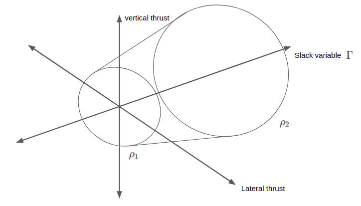
On the one hand, we have introduced a new time-varying quantity, and have thus increased the complexity of our problem. However, by introducing this quantity, we have made our constraints convex. This trade-off will be well worth it.
We can get around the nonconvex division by mass with a change of variables:
\[\sigma \equiv \frac{\Gamma}{m} \qquad \boldsymbol{u} \equiv \frac{\boldsymbol{T}_c}{m} \qquad z \equiv \ln m\]
This simplifies our dynamics to:
\[\dot{\boldsymbol{x}}(t) = \boldsymbol{A} \boldsymbol{x}(t) + \boldsymbol{B} \left(\boldsymbol{g} + \boldsymbol{u}(t)\right)\]
\[ \dot{z}(t) = -\alpha \sigma(t) \]
Unfortunately, our thrust bounds constraint becomes nonconvex:
\[0 \leq \rho_1 e^{-z(t)} \leq \sigma(t) \leq \rho_2 e^{-z(t)}\]
We can convexify it by approximating the constraint with a 2nd-order Taylor expansion of \(e^{-z(t)}\):
\[\rho_1 e^{-z_o(t)} \left(1 – (z(t) – z_o(t)) + \frac{1}{2}(z(t) – z_o(t))^2\right) \leq \sigma(t) \leq \rho_2 e^{-z_o(t)} \left(1 – (z(t) – z_o(t)) \right)\]
where \(z_o(t) = \ln (m_\text{wet} – \alpha \rho_2 t)\).
The left-hand side forms a second-order cone constraint, which have the form \(\|x\|_2 \leq t\). Quadratic constraints can be converted to such second-order cone constraints.
We thus end up with the following convex problem:
\[\begin{matrix}\text{minimize}_{\boldsymbol{u}, \boldsymbol{\sigma}} & \int_0^{t_f} \sigma(t) \> dt & & \\ \text{subject to} & \dot{\boldsymbol{x}}(t) = \boldsymbol{A} \boldsymbol{x}(t) + \boldsymbol{B} \left(\boldsymbol{g} + \boldsymbol{u}(t)\right) & \text{for all } t \in [0, t_f] & \text{physical dynamics} \\ & \dot{z} = -\alpha \sigma(t) & \text{for all } t \in [0, t_f] & \text{mass dynamics} \\ & \|\boldsymbol{u}(t)\| \leq \sigma(t) & \text{for all } t \in [0, t_f] & \text{slack variable bound} \\ & \rho_1 e^{-z_o(t)} \left(1 – (z(t) – z_o(t)) + \frac{1}{2}(z(t) – z_o(t))^2\right) \leq \sigma(t) & \text{for all } t \in [0, t_f] & \text{thrust magnitude, lower} \\ & \sigma(t) \leq \rho_2 e^{-z_o(t)} \left(1 – (z(t) – z_o(t)) \right) & \text{for all } t \in [0, t_f] & \text{thrust magnitude, upper} \\ & u_y(t) \geq \sigma(t) \cos(\theta) & \text{for all } t \in [0, t_f] & \text{thrust pointing constraint} \\ & r_y(t) \geq \tan(\gamma_\text{gs}) r_x(t)& \text{for all } t \in [0, t_f] & \text{glide slope constraint} \\ & \boldsymbol{r}(0) = \boldsymbol{r}_0, \dot{\boldsymbol{r}}(0) = \dot{\boldsymbol{r}}_0 & & \text{physical initial conditions} \\ & z(0) = \ln m_\text{wet} & & \text{mass initial condition} \\ & \boldsymbol{r}(t_f) = [0,0], \dot{\boldsymbol{r}}(t_f) = [0,0] & & \text{physical final conditions} \\ & z(t_f) \geq \ln m_\text{dry} & & \text{mass final condition} \end{matrix}\]
It can be shown that if there is a feasible solution to the first problem, then that solution also defines a feasible solution to this new problem. Furthermore, this solution is an optimal solution of the new problem. (This is related to the fact that \(\boldsymbol{u}\) is not minimized – we only care about minimizing \(\boldsymbol{\sigma}\), but for physical feasibility we end up needing \(\boldsymbol{u} = \boldsymbol{\sigma}\)).
Discretization in Time
The final problem transformation involves moving from a continuous formulation to a discrete formulation, such that we can actually implement a numerical algorithm. We discretize time into \(n\) equal-width periods such that \(n \Delta t = t_f\):
\[t^{(k)} = k \Delta t, \qquad k = 0, \ldots, n\]
Our thrust profile is a continuous function of time. We construct it as a combination of \(n+1\) basis functions, \(\phi_{0:n}\):
\[\begin{bmatrix}\boldsymbol{u}(t) \\ \sigma(t)\end{bmatrix} = \sum_{k=0}^n \boldsymbol{p}^{(k)} \phi^{(k)}(t), \qquad t \in [0,t_f]\]
where the \(\boldsymbol{p}^{(k)} \in \mathbb{R}^3\) are mixing weights that we will optimize. Note that we did not have to have as many basis functions as discrete points – it just makes the math easier. Various basis functions can be used, but the paper
\[\phi_j(t) = \begin{cases} \frac{t_j-t}{\Delta t} & \text{for } t \in [t_{j-1}, t_j] \\ \frac{t – t_j}{\Delta t} & \text{for } t \in [t_{j}, t_{j+1}] \\ 0 & \text{otherwise} \end{cases}\]
Our system state is \([\boldsymbol{r}(t)^\top, \dot{\boldsymbol{r}}(t)^\top, z(t)]^\top\)
\[\begin{split} \begin{bmatrix} \dot{\boldsymbol{r}}(t) \\ \ddot{\boldsymbol{r}}(t) \\ \dot{z}(t) \end{bmatrix} & = \begin{bmatrix} \boldsymbol{0} & \boldsymbol{I} & 0 \\ \boldsymbol{0} & \boldsymbol{0} & 0 \\ 0 & 0 & 0 \end{bmatrix} \begin{bmatrix} \boldsymbol{r}(t) \\ \dot{\boldsymbol{r}}(t) \\ z(t) \end{bmatrix} + \begin{bmatrix} \boldsymbol{0} & \boldsymbol{0} \\ \boldsymbol{I} & \boldsymbol{0} \\ 0 & -\alpha \end{bmatrix} \begin{bmatrix} \boldsymbol{u}(t) \\ \sigma(t) \end{bmatrix} + \begin{bmatrix} \boldsymbol{0} \\ \boldsymbol{g} \\ 0 \end{bmatrix} \\ \dot{\mathtt{x}(t)} & = \boldsymbol{A}_c \mathtt{x}(t) + \boldsymbol{B}_c \mathtt{u}(t) + \mathtt{g} \end{split} \]
In order to discretize, we would like to have a linear equation to get our state at every discrete time point. We know that the solution to the ODE \(\dot{x} = a x + b u\) is:
\[ x(t) = e^{at} x_0 + \int_0^t e^{A(t-\tau)} b u(\tau) \> d\tau \]
Similarly, the solution to our ODE is:
\[ \mathtt{x}(t) = e^{\boldsymbol{A_c}t} \mathtt{x}_0 + \int_0^t e^{\boldsymbol{A_c}(t-\tau)} \left(\boldsymbol{B}_c \mathtt{u}(\tau) + \mathtt{g}\right) \> d\tau \]
We can get our discrete update by plugging in \(\Delta t\):
\[ \mathtt{x}(\Delta t) = e^{\boldsymbol{A_c}\Delta t} \mathtt{x}_0 + \int_0^{\Delta t} e^{\boldsymbol{A_c}(\Delta t-\tau)} \left(\boldsymbol{B}_c \mathtt{u}(\tau) + \mathtt{g}\right) \> d\tau \]
If we’re going from \(k\) to \(k+1\), we get:
\[ \mathtt{x}^{(k+1)} = e^{\boldsymbol{A_c}\Delta t} \mathtt{x}^{(k)} + \int_0^{\Delta t} e^{\boldsymbol{A_c}(\Delta t-\tau)} \left(\boldsymbol{B}_c \mathtt{u}(\tau) + \mathtt{g}\right) \> d\tau \]
We then substitute in our
\[ \begin{split} \mathtt{x}^{(k+1)} &= \left[e^{\boldsymbol{A_c}\Delta t}\right] \mathtt{x}^{(k)} + \int_0^{\Delta t} e^{\boldsymbol{A_c}(\Delta t-\tau)} \left(\boldsymbol{B}_c \left( \boldsymbol{p}^{(k)} \phi^{(k)}(t) + \boldsymbol{p}^{(k+1)} \phi^{(k+1)}(t) \right) + \mathtt{g}\right) \> d\tau \\ & = \left[e^{\boldsymbol{A_c}\Delta t}\right] \mathtt{x}^{(k)} + \int_0^{\Delta t} e^{\boldsymbol{A_c}(\Delta t-\tau)} \left(\boldsymbol{B}_c \left( \left( 1- \frac{\tau}{\Delta t}\right) \boldsymbol{p}^{(k)} + \left( \frac{\tau}{\Delta t}\right) \boldsymbol{p}^{(k+1)} \right) + \mathtt{g}\right) \> d\tau \\ & = \left[e^{\boldsymbol{A_c}\Delta t}\right] \mathtt{x}^{(k)} + \left[\int_0^{\Delta t} e^{\boldsymbol{A_c}(\Delta t-\tau)} \boldsymbol{B}_c\right] \left( \boldsymbol{p}^{(k)} + \mathtt{g} \right) + \left[\int_0^{\Delta t} e^{\boldsymbol{A_c}(\Delta t-\tau)} \boldsymbol{B}_c \frac{\tau}{\Delta t}\right] \left( \boldsymbol{p}^{(k+1)} – \boldsymbol{p}^{(k)} \right) \\ &= \boldsymbol{A}_d \texttt{x}^{(k)} + \boldsymbol{B}_{d1} \left( \boldsymbol{p}^{(k)} + \mathtt{g} \right) + \boldsymbol{B}_{d2} \left( \boldsymbol{p}^{(k+1)} – \boldsymbol{p}^{(k)} \right) \end{split} \]
We can compute our matrices once using numerical methods for integration. We can apply our relation recursively to get our state at any discrete time point. All of these updates are linear:
\[\begin{split} \mathtt{x}^{(1)} & = \boldsymbol{A}_d \texttt{x}^{(0)} + \boldsymbol{B}_{d1} \left( \boldsymbol{p}^{(0)} + \mathtt{g} \right) + \boldsymbol{B}_{d2} \left( \boldsymbol{p}^{(1)} – \boldsymbol{p}^{(0)} \right) \\ \mathtt{x}^{(2)} & = \boldsymbol{A}_d \texttt{x}^{(1)} + \boldsymbol{B}_{d1} \left( \boldsymbol{p}^{(1)} + \mathtt{g} \right) + \boldsymbol{B}_{d2} \left( \boldsymbol{p}^{(2)} – \boldsymbol{p}^{(1)} \right) \\ &= \boldsymbol{A}_d \left(\boldsymbol{A}_d \texttt{x}^{(0)} + \boldsymbol{B}_{d1} \left( \boldsymbol{p}^{(0)} + \mathtt{g} \right) + \boldsymbol{B}_{d2} \left( \boldsymbol{p}^{(1)} – \boldsymbol{p}^{(0)} \right)\right) + \boldsymbol{B}_{d1} \left( \boldsymbol{p}^{(1)} + \mathtt{g} \right) + \boldsymbol{B}_{d2} \left( \boldsymbol{p}^{(2)} – \boldsymbol{p}^{(1)} \right) \\ &= \boldsymbol{A}_d^2 \texttt{x}^{(0)} + \left(\boldsymbol{B}_{d1} + \boldsymbol{A}_d \boldsymbol{B}_{d1}\right) \mathtt{g} + \left(\boldsymbol{A}_d \boldsymbol{B}_{d1} – \boldsymbol{A}_d \boldsymbol{B}_{d2} \right) \boldsymbol{p}^{(0)} + \left(\boldsymbol{B}_{d1} + \boldsymbol{A}_d \boldsymbol{B}_{d2} – \boldsymbol{B}_{d2} \right) \boldsymbol{p}^{(1)} + \boldsymbol{B}_{d2} \boldsymbol{p}^{(2)} \\ & \enspace \vdots \end{split}\]
Note that due to our choice of basis function, \(\boldsymbol{u}^{(k)} = [p_1^{(k)} p_2^{(k)}]^\top\) and \(\sigma^{(k)} = p_3^{(k)}\).
We can approximate the continuous version of our objective function:
\[ \int_0^{t_f} \sigma(t) \> dt \approx \sum_{k=0}^n p^{(k)}_3\]
We can pull all of this together and construct a discrete-time optimization problem. We optimize the vector \(\boldsymbol{\eta}\), which simply contains all of the \(\boldsymbol{p}\) vectors:
\[\boldsymbol{\eta} = \begin{bmatrix} \boldsymbol{p}^{(0)} \\ \boldsymbol{p}^{(1)} \\ \vdots \\ \boldsymbol{p}^{(n)} \end{bmatrix} \]
Our problem is:
\[\begin{matrix}\text{minimize}_{\boldsymbol{\eta}} & \sum_{k=0}^n p^{(k)}_3 & & \\ \text{subject to} & \mathtt{x}^{(k+1)} = \boldsymbol{A}_d \texttt{x}^{(k)} + \boldsymbol{B}_{d1} \left( \boldsymbol{p}^{(k)} + \mathtt{g} \right) + \boldsymbol{B}_{d2} \left( \boldsymbol{p}^{(k+1)} – \boldsymbol{p}^{(k)} \right) & \text{for all } k \in [0, 1, \ldots, n-1] & \text{dynamics} \\ & \|[p_1^{(k)} p_2^{(k)}]^\top\| \leq p_3^{(k)} & \text{for all } k \in [0, 1, \ldots, n] & \text{slack variable bound} \\ & \rho_1 e^{-z_o(k \Delta t)} \left(1 – (z(k \Delta t) – z_o(k \Delta t)) + \frac{1}{2}(z(k \Delta t) – z_o(k \Delta t))^2\right) \leq \sigma(k \Delta t) & \text{for all } k \in [0, 1, \ldots, n] & \text{thrust magnitude, lower} \\ & \sigma(k \Delta t) \leq \rho_2 e^{-z_o(k \Delta t)} \left(1 – (z(k \Delta t) – z_o(k \Delta t)) \right) & \text{for all } k \in [0, 1, \ldots, n] & \text{thrust magnitude, upper} \\ & p_2^{(k)} \geq p_3^{(k)} \cos(\theta) & \text{for all } k \in [0, 1, \ldots, n] & \text{thrust pointing constraint} \\ & r_y(k \Delta t) \geq \tan(\gamma_\text{gs}) r_x(k \Delta t)& \text{for all } k \in [0, 1, \ldots, n-1] & \text{glide slope constraint} \\ & \boldsymbol{r}(0) = \boldsymbol{r}_0, \dot{\boldsymbol{r}}(0) = \dot{\boldsymbol{r}}_0 & & \text{physical initial conditions} \\ & z(0) = \ln m_\text{wet} & & \text{mass initial condition} \\ & \boldsymbol{r}(t_f) = [0,0], \dot{\boldsymbol{r}}(t_f) = [0,0] & & \text{physical final conditions} \\ & z(t_f) \geq \ln m_\text{dry} & & \text{mass final condition} \end{matrix}\]
This final formulation is a finite-dimensional second-order cone program (SOCP). It can be solved by standard convex solvers to get a globally-optimal solution.
Note that we only apply our constraints at the discrete time points. This tends to be sufficient, due to the linear nature of our dynamics.
Coding it Up
cvxpy. My python notebook is available here.
Update: I originally did the implementation in Julia, but found odd behavior with the Convex.jl solvers I was using. I tried both SCS (the default recommended solver for Convex.jl) and COSMO. Neither of these solvers worked for the propulsive landing problem. Both solvers had the same behavior – they would find a solution that satisfied the terminal conditions, but would fail to satisfy the other constraints. Giving it more iterations would cause it to slowly make progress on the other constraints, but eventually it would give up and decide the problem is infeasible.
Prof. Kochenderfer noticed that Julia didn’t work for me, and recommended that I try ECOS. I swapped that in and it just worked. My Julia notebook is available here.
import cvxpy as cp
import numpy as np
import scipy
We define our parameters, which I adapted from the paper:
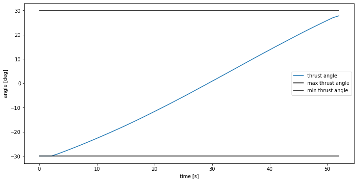
m_wet = 2000.0        # rocket wet mass [kg]
m_dry =  300.0        # rocket dry mass [kg]
thrust_max = 24000.0  # maximum thrust
ρ1 = 0.2 * thrust_max # lower bound on thrust
ρ2 = 0.8 * thrust_max # upper bound on thrust
α = 5e-4              # rocket specific impulse [s]
θ = np.deg2rad(30)    # max thrust angle deviation from vertical [rad]
γ = np.deg2rad(15)    # no-fly bounds angle [rad]
g = 3.71              # (martian) gravity [m/s2]
tf = 52.0             # duration of the simulation [s]
n_pts = 50            # number of discretization points

# initial state (x,y,x_dot,y_dot,z)
x0 = np.array([600.0, 1200.0, 50.0, -95.0, np.log(m_wet)])
We then compute some derived parameters:
t = np.linspace(0.0, tf, n_pts) # time vector [s]
N = len(t) - 2                  # number of control nodes
dt = t[1] - t[0]
We compute \(\boldsymbol{A}_c\) and \(\boldsymbol{A}_d\):
Ac = np.vstack((
        np.hstack((np.zeros((2, 2)), np.eye(2),        np.zeros((2, 1)))),
        np.hstack((np.zeros((2, 2)), np.zeros((2, 2)), np.zeros((2, 1)))),
        np.zeros((1, 5))
     ))

Ad = scipy.linalg.expm(Ac * dt)
We compute \(\boldsymbol{B}_c\), \(\boldsymbol{B}_{d1}\), and \(\boldsymbol{B}_{d2}\):
def integrate_trapezoidal(f, a, b, n):
    retval = f(a) * 0.5 + f(b) * 0.5
    for k in range(1, n):
        retval = retval + f(a + k*(b-a)/n)
    retval = retval * (b - a)/ n
    return retval

Bc = np.vstack((
        np.hstack((np.zeros((2, 2)), np.zeros((2, 1)))),
        np.hstack((np.eye(2),        np.zeros((2, 1)))),
        np.hstack((np.zeros((1, 2)), np.reshape(np.array([-α]), (1, 1))))
    ))

Bd1 = integrate_trapezoidal(lambda s: np.matmul(scipy.linalg.expm(Ac*(dt-s)), Bc), 0.0, dt, 10000)
Bd2 = integrate_trapezoidal(lambda s: np.matmul(scipy.linalg.expm(Ac*(dt-s))*(s/dt), Bc), 0.0, dt, 10000)
We implement our recursive calculation for the state at time index \(k\):
# gravitational 3-vector [m/s2]
g3 = np.array([0.0, -g, 0.0])

def get_xk(Ad, Bd1, Bd2, η, x0, g3, k):
    xk = x0
    p_km1 = np.array([0.0,0.0,0.0])
    p_k = η[0:3]
    ind_low = 0
    for j in range(0,k):
        xk = np.matmul(Ad,xk) + np.matmul(Bd1, (p_km1 + g3)) + np.matmul(Bd2, (p_k - p_km1))
        p_km1 = p_k
        ind_low = min(ind_low+3, 3*(N+1))
        p_k = η[ind_low : ind_low+3]
    return xk
and we define our problem:
# Create the CVX problem
η = cp.Variable(3*N)

ω = np.tile(np.array([0,0,1]), N) # only minimize the σ's

# minimize fuel consumption
objective = cp.Minimize(ω.T@η)
constraints = []

# thrust magnitude constraints
for k in range(0, N):
    j = 3*k
    constraints.append(cp.norm(η[j:j+2]) <= η[j+2])

# thrust cant angle constraints
for k in range(0, N):
    j = 3*k
    uy = η[j+1]
    σ = η[j+2]
    constraints.append(uy >= np.cos(θ) * σ)

# thrust slack variable lower and upper bounds
z0 = lambda k: np.log(m_wet - α*ρ2*dt*k)
for k in range(0, N):
    j = 3*k
    σk = η[j+2]
    xk = get_xk(Ad, Bd1, Bd2, η, x0, g3, k)
    zk = xk[-1]

    a = ρ1 * np.exp(-z0(k))
    z0k = z0(k).item()
    z1k = z1(k).item()

    constraints.append(a * (1 - (zk-z0k) + 0.5*cp.square(zk-z0k)) <= σk)
    constraints.append(σk <= ρ2 * np.exp(-z0k) * (1 - (zk-z0k)))

# glide angle constraints
for k in range(1, N):
    j = 3*k
    xk = get_xk(Ad, Bd1, Bd2, η, x0, g3, k)
    constraints.append(xk[1] >= np.tan(γ) * xk[0])

# terminal conditions
xf = get_xk(Ad, Bd1, Bd2, η, x0, g3, N)
constraints.append(xf[0:4] == [0,0,0,0])
constraints.append(xf[4] >= np.log(m_dry))

prob = cp.Problem(objective, constraints)
and we solve it!
result = prob.solve()
print(prob.status)
We can extract our solution (thrust profile and trajectory) as follows:
η_eval = η.value

xk = np.zeros((len(x0), len(t)))
for (i,k) in enumerate(range(0,N)):
    xk[:,i] = get_xk(Ad, Bd1, Bd2, η_eval, x0, g3, k)

xs = xk[0,:]
ys = xk[1,:]
us = xk[2,:]
vs = xk[3,:]
zs = xk[4,:]

mass = np.exp(zs)

u1 = η_eval[0::3]
u2 = η_eval[1::3]
σ = η_eval[2::3]

Tx = u1 * mass
Ty = u2 * mass
Γ = σ * mass
thrust_mag = [np.hypot(Tyi, Txi) for (Txi, Tyi) in zip(Tx, Ty)]
thrust_ang = [np.arctan2(Txi, Tyi) for (Txi, Tyi) in zip(Tx, Ty)]
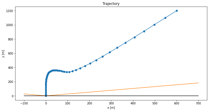
The plots end up looking pretty great. Here is the landing trajectory we get for the code above:
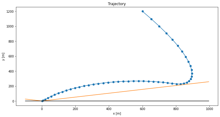
The blue line shows the rocket’s position over time, the orange line shows the no-fly boundary, and the black line shows the ground (\(y = 0\)). The rocket has to slow down so as to avoid the no-fly zone (orange), and then nicely swoops in for the final touchdown. Here is the thrust profile:

Our thrust magnitude matches our slack variable \(\Gamma\), as expected for optimal trajectories. We also see how the solution “rides the rails”, hitting both the upper and lower bounds. This is very common for optimal control problems – we use all of the control authority available to us.
The two thrust components look like this:
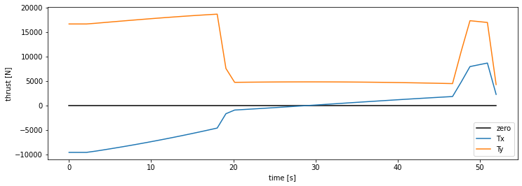
We see that \(T_y\) stays positive, as it should. However, \(T_x\) starts off negative to move the rocket left, and then counters in order to stick the landing.
Our thrust angle stays within bounds:
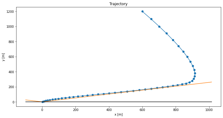
We can of course play around with our parameters and initial conditions to get different trajectories. Here is what happens if we flip the initial horizontal velocity:
Here is what happens if we increase the minimum thrust to \(\rho_1 = 0.3 T_\text{max}\):
How to Avoid Specifying the Trajectory Duration
One remaining issue with the convex formulation above is that we have to specify our trajectory duration, \(t_f\). This, and \(n\), determine \(\Delta t\) and our terminal condition, both of which are pretty central to the problem.
We might be interested, for example, in finding the minimum-time landing trajectory. Typically, the longer the trajectory, the more fuel that is used, so being able to reduce \(t_f\) automatically can have big benefits.
The naive approach is to do a search over \(t_f\) in order to find the smallest valid trajectory duration. In fact, this is exactly what the authors suggest:
Once we have a procedure to compute the fuel optimal trajectory for a given time-of-flight, \(t_f\), we use the Golden search algorithm to determine the time-of-flight with the least fuel need, \(t^*_f\). This line search algorithm is motivated by the observation that the minimum fuel is a unimodal function of time with a global minimum
Behcet Acikmese, Lars Blackmore, Daniel P. Scharf, and Aron Wolf
I would be surprised if there were a way to optimize for \(t_f\) alongside the trajectory, but there very well could be a better approach!
The Curious Case of the Missing Constraint
As a final note, I wanted to mention that there are some additional constraints in some versions of the paper. Notably, this paper includes these constraints in its “Problem 3”:
\[ \log\left(m_\text{wet} – \alpha \rho_2 t\right) \leq z(t) \leq \log\left(m_\text{wet} – \alpha \rho_1 t\right) \]
These constraints do not appear in Lossless Convexification of Nonconvex Control Bound and Pointing Constraints of the Soft Landing Optimal Control Problem.
After thinking about it, I don’t think the constraints are needed. They are enforcing that our mass lies between an upper and lower bound. The upperbound is the mass we would have if we had minimum thrust for the entire trajectory, whereas the lowerbound is the mass we would have if we had maximum thrust for the entire trajectory. The fact that we constrain our thrusts (and constrain our final mass) mean that we don’t really need these constraints.
Conclusion
I find this problem fascinating. We go through a lot of math, so much that it can be overwhelming, but it all works out in the end. Every step ends up being understandable and justifiable. I then love seeing the final trajectories play out, and get the immediate feedback in the trajectory as we adjust the initial conditions and constraints.
I hope you enjoyed this little side project.