A Transformer Sokoban Policy

I’ve posted about Sokoban before. It is a problem I keep coming back to.

Sokoban is both very simple to specify but its difficulty can be readily scaled up. It is easy to accidentally push blocks into an inescapable kerfuffle, and more interestingly, it isn’t always obvious when you’ve done it.

Moreover, I think people solving Sokoban often beautifully exhibit hierarchical reasoning. The base game is played with up/down/left/right actions, but players very quickly start thinking about sequences of block pushes. We learn to “see” deadlock configurations and reason about rooms and packing orders. This ability to naturally develop higher-order thinking and execute on it is something I want to understand better. So I keep coming back to it.

In this blog post, I’ll recount training a Sokoban policy using deep learning, and more specifically, using the transformer architecture. I started pretty small, developing something I that hope to flesh out more in the future.

The Problem

This blog post is about policy optimization. A policy \(\pi(s)\) maps states to actions. These states and actions must exist in some sort of problem — i.e. a search problem or Markov decision process. It is often a good idea to define the problem before talking about how to structure the policy.

Our problem, of course, is Sokoban. The state space is the space of Sokoban boards. Each board is a grid, and each tile in the grid is either a wall or a floor, each floor may be a goal and may contain either a box or the player. For this post I’m working with 8×8 boards.

\[\text{state space}\enspace\mathcal{S} = \text{Sokoban boards}\]

Normal Sokoban has an action space of up/down/left/right. At least, that is what we’re told. I think that isn’t quite true. In normal Sokoban, the player can get stuck in a deadlock. When that happens, they typically reset the level or hit undo. So I’m going use an action space of up/down/left/right/undo. Trajectories with undos are of course never optimal, but you nevertheless might need to use them when you’re exploring.

\[\text{action space}\enspace\mathcal{A} = \left\{\text{up}, \text{down}, \text{left}, \text{right}, \text{undo}\right\}\]

Notice that we’re working directly with player movements, not with box pushes. Pretty much no-one ever works directly with player movements, because the search space gets so large so quickly. That being said, hierarchical reasoning is the point of my investigations, so I’m starting at the bottom of the reasoning hierarchy.

Our goal is to solve Sokoban problems. For now, let’s just say that we get a reward of 1 whenever we solve a board (all boxes are on goals), and zero reward otherwise. Given two action sequences that solve a board, we prefer the shorter one.

\[R(s,a) = \begin{cases}1 & \text{if } \texttt{issolved}(s) \\ 0 & \text{otherwise}\end{cases}\]

We won’t directly make use of this reward function in this blog post, but it will come into play later.

The Policy

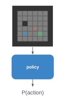
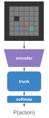
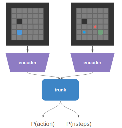
A typical policy would take the current state and try to find the best action that leads toward having all boxes on goals. Its architecture would broadly look like:

The output is a probability distribution over the actions. There are 5 actions (up,down,left,right, and undo), so this is just a categorical distribution over 5 values. That’s the bread and butter of ML and we can easily produce that with a softmax output layer.

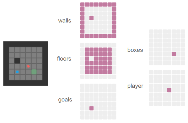
The input is a board state. I decided to represent boards as \(8\times 8\times 5\) tensors, where the first two dimensions are the board length and width, and then we have 5 channels that indicate whether a given tile is a wall space, a floor space, has a goal, has a player, and has a box. Altogether that is 320 scalars, which is somewhat long and sparse. However, it contains a lot of structured spatial information that we need to make use of.

The first architectural decision is to run the board state through an encoder head to produce a latent vector. Its basically a 5-channel image, so I’m using convolutional layers, just like you would for an image input. These can learn consistent features that get applied in parallel across the input.

This could work. We’d just stick some feedforward layers with maybe some residual connections into that trunk, and we’d be able to train a policy to place all boxes on goals. I didn’t quite want to go that route though, because I wanted the network to be slightly more configurable.

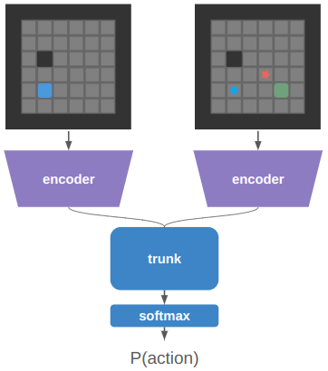
My eventual goal is to do hierarchical reasoning, so I want to be able to have another, higher-level policy use this lower-level policy as a tool. As such, I want an input that it can provide in order to steer the policy. To this end, I’m providing an additional goal input that tells the neural network what we want to happen:

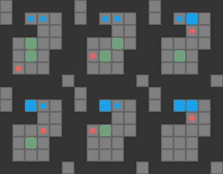
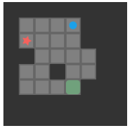
In Sokoban its pretty important for the player to know when a board just isn’t solvable. Its really easy to end up in a deadlock state:

We want the model to be able to learn when this happens, and to be able to report that it thinks this is the case.

I thus include an additional output, which I’m calling the nsteps output. It predicts the number of steps left in the solution of the puzzle. If the network thinks there are an infinite number of steps left, then the board is not solvable.

In Stop Regressing, the authors suggest avoiding (continuous) regression and to train over discrete targets instead. As such, my nsteps output will actually output a discrete value:

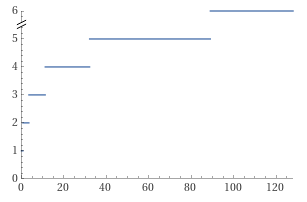
nsteps = Int(clamp(round(log(nsteps+1)), 0, 5)) + 1

which can take on up to 6 values:

and a 7th bin for unsolvable.

That leaves our network as (with the softmaxes implied):

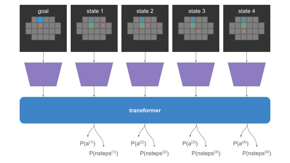
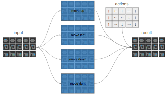
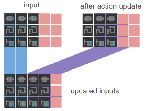
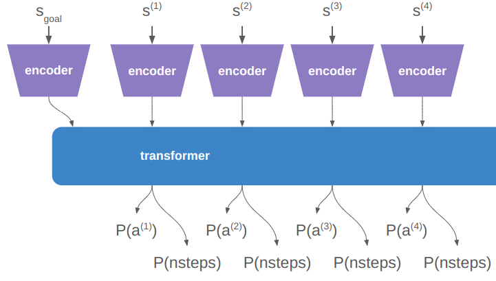
This architecture is a perfectly reasonable policy network. In fact, we’ll compare against this network later on. However, I was also very interested in working with transformers, so I built a transformer version of this network:

This architecture is roughly the same, except you have the massively parallel transformer that:

  • can train with supervised learning more efficiently, by receiving an entire sequence at once
  • can use past information to inform future decisions
  • can easily be scaled up or down based on just a few parameters
  • lends itself nicely to beam search for exploration

I am initially working with relatively small models consisting of 3-layer transformers with 16-dimensional embedding spaces, a maximum sequence length of 32, and 8-headed attention.

Training

This initial model is trained with supervised learning. In order to do that, we need supervised data.

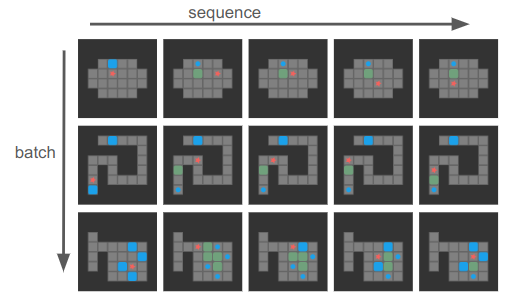
Typical supervised learning would provide a starting state, the goal state, and an optimal set of actions to reach it. My training examples are basically that, but also include examples that cannot be solved and some examples with bad moves and a training mask that allows me to mask them out during training. (This theoretically lets the network learn undos and to recover from bad moves).

start:
########
# #
# #
# . bp #
# #
# #
# #
########

goal:
########
# #
# #
# B #
# #
# #
# #
########

solved
moves: LL
isbad: --

solved
moves: xLL
isbad: x--


solved
moves: UxLL
isbad: xx--

I have a few handcrafted training entries, but most of them are randomly generated problems solved with A*. I generate 1-box problems by starting with an 8×8 grid of all-walls, producing two random rectangular floor sections (rooms), randomly spawning the goal, box, and the player, and then speckling in some random walls. That produces a nice diversity that has structure, but not too much structure.

Most of these boards aren’t solvable, so I when I generate training examples, I set a target ratio for solved and unsolved boards and make sure to keep generating until I get enough of each type. I have 4000 generated problems with solutions and 4000 generated problems without solutions, resulting in 8,000 overall generated training examples.

I was able to cheaply boost the size of the training set by recognizing that a problem can be rotated 4 ways and can be transposed. Incorporating these transforms (and applying the necessary adjustments to the solution paths) automatically increases the number of training examples by 8x.

I train with a standard Flux.jl loop using the default Adam optimizer. I shuffle the training set with each epoch, and train with a batch size of 32. I’m using 1% dropout.

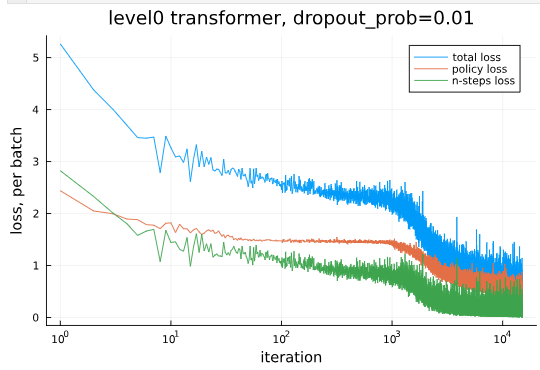
The training loop is set up to create a new timestamped directory with each run and save a .json file with basic metrics. I compute both the policy and nsteps loss on each batch and log these for later printing. This gives me nice training curves, effectively using the code from the Flux quick start guide:

This plot uses a log-scale x-axis, which gives it some distortion. Training curves are often plotted this way because a lot of stuff happens early on and more updates have to be be made later on to get similar movement.

I’ve been consistently seeing the plots play out like they do above. At first the loss drops very quickly, only to plateau between 100 and 1000 batches, and then to suddenly start reducing again. The model seems to suddenly understand something around the 1000-batch mark. Based on how flat the policy loss is, it seems to be related to that. Maybe it learns some reliable heuristics around spatial reasoning and walking to boxes.

The curves suggest that I could continue to train for longer and maybe get more improvement. Maybe that’s true, and maybe I’ll look into that in the future.

Validation

I have two types of validation – direct supervised metrics and validation metrics based on using the policy to attempt to solve problems. Both of these are run on a separate validation dataset of 4000 randomly generated problems (with a 50-50 split of solvable and not solvable).

The supervised metrics are:

  • accuracy at predicting whether the root position is solvable
  • top-1 policy accuracy – whether the highest-likelihood action matches the supervised example
  • top-2 policy accuracy – whether the supervised example action is in the top two choices
  • top-1 nsteps accuracy – whether the highest-likelihood nsteps bucket matches the example
  • top-2 nsteps accuracy – ditto, but top two choices

Note that a Sokoban problem can have multiple solutions, so we shouldn’t expect a perfect policy accuracy. (i.e. going up and then left is often the same as going left and then up).

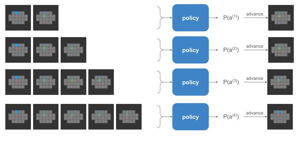
I then use the model to solve each problem in the validation dataset using beam search. This lets me actually test efficacy. Beam search was run with a beam width of 32, which means I’m always going to find the solution if it takes fewer than 2 steps. The search keeps the top candidates based on the running sum of the policy likelihood. (I can try other formulations, like scoring candidates based on the predicted nsteps values).

Results

I trained two models – a transformer model and a 2nd model that does not have access to past data. The 2nd model is also a transformer, but with a mask that masks out everything but the current and goal states.

The metrics are:

TransformerBaseline
Solvability Accuracy0.9770.977
Top-1 Policy Accuracy0.8670.831
Top-2 Policy Accuracy0.9820.969
Top-1 Nsteps Accuracy0.9000.898
Top-2 Nsteps Accuracy0.9900.990
Solve Rate0.9210.879
Mean Solution Length6.9836.597

Overall, that’s pretty even. The baseline policy that does not have access to past information is ever so slightly worse with respect to top-1 accuracy. Our takeaway is that for this problem, so far, the past doesn’t matter all that much and we can be pretty Markovian.

A 97.7% solvability accuracy is pretty darn good. I am happy with that.

The top-k policy and nsteps accuracies are pretty good too. The full transformer outperforms the baseline a bit here, but only by a bit.

The primary difference comes out when we look at the solve rate, which we obtain by actually using the policies to solve problems. The full transformer succeeds 92.1% of the time, whereas when there is no history it only solves it 87.9% of the time. That’s only a 4.2% spread, but it is noticeable. I can only hypothesize, but I suspect past information is useful for longer traversals and simply the fact that you can pull more information in can give the model more space to compute with.

Transformers – How and Why They Work

This month I decided to take a break from my sidescroller project and instead properly attend to transformers (pun intended). Unless you’ve been living under a rock, you’ve noticed the rapid advanced of AI in the last year and the advent of extremely large models like ChatGPT 4 and Google Gemini. These models, and pretty much every other large and serious application of AI nowadays, are based on the transformer architecture first introduced in Attention is All You Need. So this post is about transformers, how and roughly why they work, and how to write your own.

The Architecture

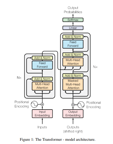
The standard depiction of the transformer architecture comes from Figure 1 of Attention is All You Need:

I initially found this image difficult to understand. Now that I’ve implemented my own transformer from scratch, I’m actually somewhat impressed by its concise expressiveness. That’s appropriate for a research paper where information density is key, but I think we can do better if we’re explaining the architecture to someone.

Transformers at base operate on tokens, which are just discrete items. In effect, if you have 5 tokens, then you’re talking about having tokens 1, 2, 3, 4, and 5. Transformers first became popular when used on text, where tokens represents words like “potato” or fragments like “-ly”, but they have since been applied to chunks of images, chunks of sound, simple bits, and even discrete states, actions, and rewards. I think words are the most intuitive to work with, so let’s go with that.

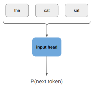
Transformers predict the next token some given all of the tokens that came before:

\[P(x_{t} \mid x_{t-1}, x_{t-2}, \ldots)\]

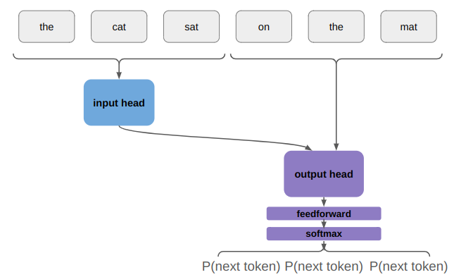
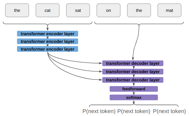
For example, if we started a sentence with “the cat sat”, we might want it to produce a higher likelihood for “on” than “potato”. Conceptually, this looks like:

The output probability distribution is just a Categorical distribution over the \(n\) possible tokens, which we can easily produce with a softmax layer.

You’ll notice that my model goes top to bottom whereas academia for some unfathomable reason usually depicts deep neural nets bottom to top. We read top to bottom so I’m sticking with that.

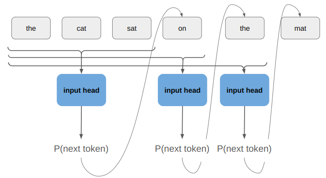
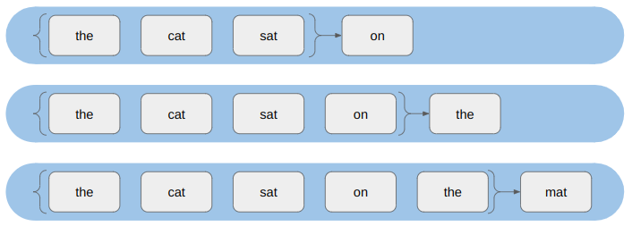
We could use a model like this to recursively generate a full sentence:

So far we’ve come up with a standard autoregressive model. Those have been around forever. What makes transformers special is that they split the inputs from the outputs such that the inputs need only be encoded once, that they use attention to help make the model resilient to how the tokens are ordered, and that they solve the problem of vanishing gradients.

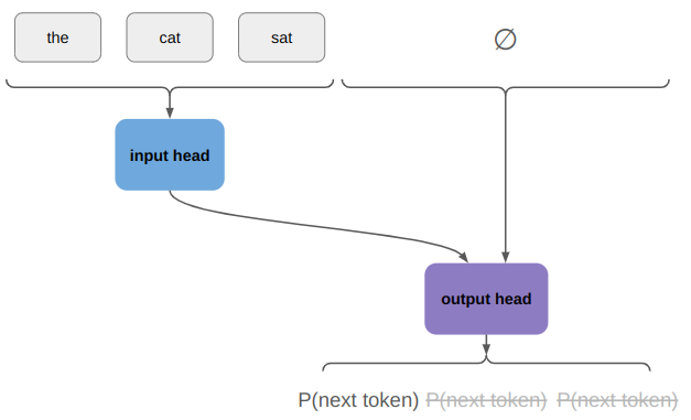
Separate Inputs and Outputs

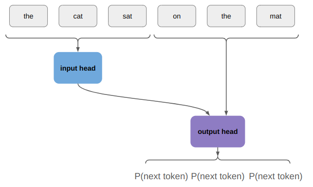
The first weird thing about the transformer architecture figure is that it has a left side and a right side. The left side receives “inputs” and the right side receives “outputs”. What is going on here?

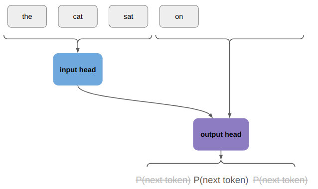
If we are trying to generate a sentence that starts with “the cat sat”, then “the cat sat” is the inputs and the subsequent tokens are the outputs. During training we’d know what the subsequent tokens are (our training set would split sentences into (input, output) pairs, such as randomly in the middle or via question/answer), and during inference we’d sample the outputs sequentially.

Conceptually, we’re now thinking about an architecture along these lines:

Is this weird? Yes. Why do they do it? Because it’s more efficient during training, and during inference you only need to run the input head once.

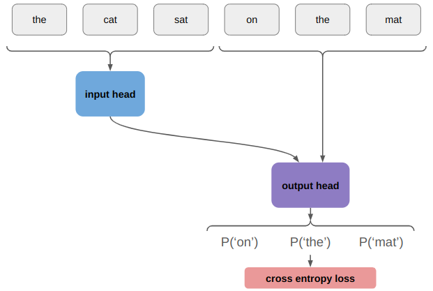
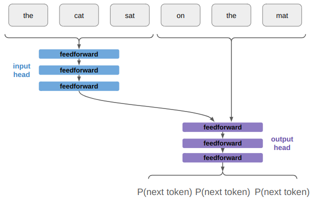
During training, we know all of the tokens and so we just stick a loss function on this to maximize the likelihood of the correct output token:

During inference, we run the encoder once and start by running the model with an empty output:

We only use the probability distribution over the first token, sample from it, and append the sampled token to our output. If we haven’t finished out sentence yet, we continue on:

We only use the probabilistic distribution over the next token, sample from it, etc. This iterative process is auto-regressive, just like we were talking about before. (aside 1) (aside 2)

The reason I think this approach is awkward is because you’d typically want the representation of \(P(x_{t} \mid x_{t-1}, x_{t-2}, \ldots)\) to not care about whether the previous tokens were original inputs or not. That is, we want \(P(\text{the} | \text{the cat sat on})\) to be the same irrespective of whether “the cat sat on” are all inputs or whether “the cat sat” is the input and we just sampled “on”. In a transformer, they are different.

Robust to Token Ordering

The real problem that the transformer architecture solves is a form of robustness to token ordering. Let’s consider the following two input / output pairs:

  • the cat sat | on the mat
  • the yellow cat sat | on the mat

They are the same except for the extra “yellow” token in the second sentence.

If our model was made up of simple feed-forward layers, that would present a problem:

A feedforward layer contains an affine transform \(\boldsymbol{x}’ \gets \boldsymbol{A} \boldsymbol{x} + \boldsymbol{b}\) that learns a different mapping for every input. We can even write it out for three inputs:

\[\begin{matrix}x’_1 &\gets A_{11}x_1 + A_{12}x_2 + A_{13}x_3 + b_1 \\ x’_2 &\gets A_{21}x_1 + A_{22}x_2 + A_{23}x_3 + b_2 \\ x’_3 &\gets A_{31}x_1 + A_{32}x_2 + A_{33}x_3 + b_3\end{matrix}\]

If we learn something about “cat” being in the second position, we’d have to learn it all over again to handle the case where “cat” is in the third position.

Transformers are robust to this issue because of their use of attention. Put very simply, attention allows the neural network to learn when particular tokens are important in a position-independent way, such that they can be focused on when needed.

Transformers use scaled dot product attention. Here, we input three things:

  • a query \(\boldsymbol{q}\)
  • a key \(\boldsymbol{k}\)
  • a value \(\boldsymbol{v}\)

Each of these are vector embeddings, but they can be thought of as:

  • query – a representation of what we are asking for
  • key – how well the current token we’re looking at reflects what we’re asking for
  • value – how important it is that we get something that matches what we’re asking for

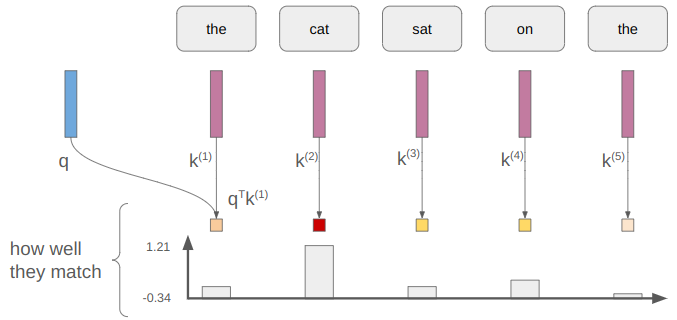
For example, if we have “the cat sat on the ____”, and we’re looking to fill in that last blank, it might be useful for the model to have learned a query for representing things that sit, and to value the result of that query a lot when we need to fill in a word for something that sits.

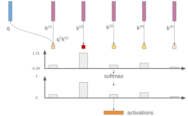
We take the dot product of the query and the key to measure how well they match: \(\boldsymbol{q}^T \boldsymbol{k}\). Each token has a key, so we end up with a measure of how well each of them matches:

Those measures can take on any values. Taking the softmax turns these measures into values that lie in [0,1], preserving relative size: (aside)

In this example, our activation vector has a large value (closer to 1) for “cat”.

Finally, we can take the dot product of our activation vector \(\boldsymbol{\alpha}\) with our value vector to get the overall attention value: \(\boldsymbol{\alpha} \cdot \boldsymbol{v}\).

Notice that where cat was in the list of tokens didn’t matter all to much. If we shift it around, but give it the same key, it will continue to produce the same activation value. Then, as long as the value is high anywhere that activation is active, we’ll get a large output.

Putting this together, our attention function for a single query \(\boldsymbol{q}\) is:

\[ \texttt{attention}(\boldsymbol{q}, \boldsymbol{k}^{(1)}, \ldots, \boldsymbol{k}^{(n)}, \boldsymbol{v}) = \texttt{softmax}\left(\boldsymbol{q}^T [\boldsymbol{k}^{(1)}, \ldots, \boldsymbol{k}^{(n)}]\right) \cdot \boldsymbol{v} \]

We can combine the keys together into a single matrix \(\boldsymbol{K}\), which simplifies things to:

\[ \texttt{attention}(\boldsymbol{q}, \boldsymbol{K}, \boldsymbol{v}) = \texttt{softmax}\left(\boldsymbol{q}^T \boldsymbol{K}\right) \cdot \boldsymbol{v} \]

We’re going to want a bunch of queries, not just one. That’s equivalent to expanding our query and value vectors into matrices:

\[ \texttt{attention}(\boldsymbol{Q}, \boldsymbol{K}, \boldsymbol{V}) = \texttt{softmax}\left(\boldsymbol{Q}^T \boldsymbol{K}\right) \boldsymbol{V} \]

We’ve basically recovered the attention function given in the paper. I just has an additional scalar term that helps keep the logits passed into softmax smaller in magnitude:

\[\texttt{attention}(\boldsymbol{Q}, \boldsymbol{K}, \boldsymbol{V}) = \texttt{softmax}\left(\frac{\boldsymbol{Q}\boldsymbol{K}^T}{\sqrt{d_k}}\right) \boldsymbol{V}\]

where \(d_k\) is the dimension of the keys — i.e. how many features long the embeddings are.

The output is a matrix that has larger entries where our queries matched tokens and our value was large. That is, the transformer learned to ask for something and extract it out if it exists.

Robust to Vanishing Gradients

The other important problem that transformers solve is the vanishing gradient problem. The previous alternative to the transformer, the recurrent neural network (RNN), tends to suffer from this issue.

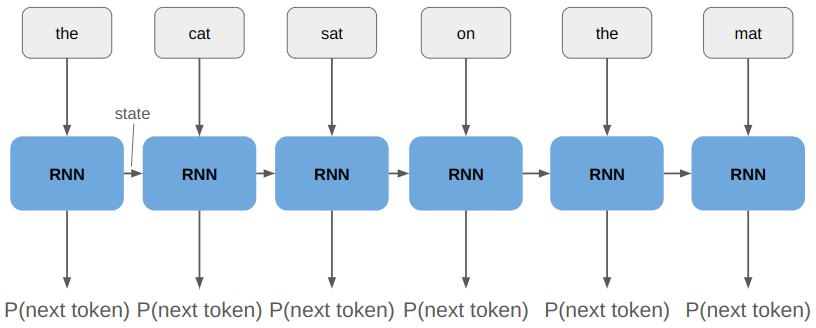
A recurrent neural network represents a sequence by taking as input the current token and a latent state:

This state is referred to as the RNN’s memory.

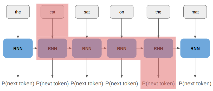
The vanishing gradients problem arises when we try to propagate gradient information far back in time (where far can just be a few tokens). If we want the network to learn to associate “mat” with “cat”, then we need to propagate through 4 instances of the RNN:

Simply put, in this example we’re taking the gradient of RNN(RNN(RNN(RNN(“cat”, state)). The chain rule tells us that the derivative of \(f(f(f(f(x))))\) is:

\[f'(x) \> f'(f(x)) \> f'(f(f(x))) \> f'(f(f(f(x))))\]

If \(f'(x)\) is smaller than 1, then we very quickly drive that gradient signal toward zero as we try to propagate it back further. The gradient vanishes!

Transformers solve this problem by having all of the inputs be mixed in the attention layers. This allows the gradient to readily flow across.

It also mitigates the problem using residual connections. These are the “skip connections” that you’ll see below. They provide a way for the gradient to flow up the network unimpeded, so it doesn’t decrease if it has to travel through a bunch of transformer layers.

Building a Transformer

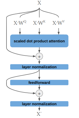
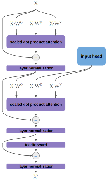
Let’s use what we’ve learned and build a transformer, setting aside the fact that we haven’t covered multiheaded attention just yet. We’re going to construct the following input head:

This is analogous to a single “input encoder layer” in the transformer architecture. Note that the real deal uses multiheaded attention and has dropout after each layer norm.

The trainable parameters in our input head are the three projection matrices \(\boldsymbol{W}^Q\), \(\boldsymbol{W}^K\), and \(\boldsymbol{W}^V\), as well as the learnable params in the feedforward layer. Layer normalization is simply normalization along each input vector rather than along the batch dimension, which keeps things nicely scaled.

I’m going to implement this input head in Julia, using Flux.jl. The code is remarkably straightforward and self-explanatory:

struct InputHead
    q_proj::Dense
    k_proj::Dense
    v_proj::Dense
    norm_1::LayerNorm
    affine1::Dense
    affine2::Dense
    norm_2::LayerNorm
end

Flux.@functor InputHead

function (m::InputHead)(
    X::Array{Float32, 3}) # [dim × ntokens × batch_size]

    dim = size(X, 1)

    # scaled dot product attention
    Q = m.q_proj(X) # [dim × ntokens × batch_size]
    K = m.k_proj(X) # [dim × ntokens × batch_size]
    V = m.v_proj(X) # [dim × ntokens × batch_size]
    α = softmax(Q*K'./√Float32(dim), dims=1)
    X′ = α*V

    # add norm
    X = m.norm_1(X + X′)

    # feedforward
    X′ = m.affine2(relu(m.affine1(X)))
    
    # add norm
    X = m.norm_1(X + X′)

    return X
end

Once we have this, building the rest of the simplified transformer is pretty easy. Let’s similarly define an output head:

The output head is basically the same, except it has an additional attention + layer normalization section that receives its query from within the head but its keys and values from the input head. This is sometimes called cross attention, and allows the outputs to receive information from the inputs. Implementing this in Julia would be pretty straightforward, so I’m not covering it here.

In order to fully flesh out a basic transformer, we just have to define what happens at the outputs and inputs. The output is pretty simple. Its just a feedforward layer followed by a softmax:

The feedforward layer both provides a chance for everything to get properly mixed (since its fully connected), but more importantly, changes the tensor dimension from the embedding size to the number tokens. The softmax then ensures that the output represents probabilities.

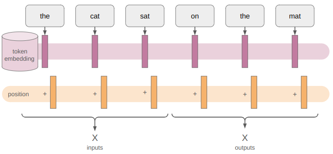
The inputs, by which I mean all of the tokens, have to be turned into embedding matrices. Remember that there’s only a finite set of tokens. We associate a vector embedding with each token, which we re-use every time the token shows up. This embedding can be learned, in which case its the same as having our token be a one-hot vector \(x_\text{one-hot}\) and learning some matrix \(m\times n\) matrix \(E\) where \(m\) is the embedding dimension and \(n\) is the number of tokens:

\[z = E x_\text{one-hot}\]

We then add a positional encoding to each embedding. Wait, I thought we wanted the network to be robust to position? Well yeah, it is. But knowing where something shows up, and whether it shows up before or after something else is also important. So to give the model a way to determine that, we introduce a sort of signature or pattern to each embedding. The original paper uses a sinusoidal pattern:

\[z_\text{pos encode}(i)_j = \begin{cases} \sin\left(i / 10000^{2j / j_\text{max}}\right) & \text{if } j \text{ is even} \\ \cos\left(i / 10000^{2j / j_\text{max}}\right) & \text{otherwise} \end{cases}\]

for the \(j\)th entry of the position encoding at position \(i\).

What I’m not showing here is that the original paper again uses dropout after the position encoding is added in.

Flux already supports token embeddings, so let’s just use that. We can just generate our position encodings in advance:

function generate_position_encoding(dim::Int, max_sequence_length::Int)
    pos_enc = zeros(Float32, dim, max_sequence_length)

    for j in 0:2:(dim-1)
        denominator::Float32 = 10000.0^(2.0*(j ÷ 2)/dim)
        for i in 1:max_sequence_length
            pos_enc[j+1, i] = sin(i / denominator)
        end
    end

    for j in 1:2:(dim-1)
        denominator::Float32 = 10000.0^(2.0*(j ÷ 2)/dim)
        for i in 1:max_sequence_length
            pos_enc[j+1, i] = cos(i / denominator)
        end
    end

    return pos_enc
end

The overall input encoder is then simply:

struct InputEncoder
    embedding::Embedding # [vocab_size => dim]
    position_encoding::Matrix{Float32} # [dim × n_tokens]
    dropout::Dropout
end

Flux.@functor InputEncoder

function (m::InputEncoder)(tokens::Matrix{Int}) # [n_tokens, batch_size]
    X = m.embedding(tokens) # [dim × n_tokens × batch_size]
    X = X .+ m.position_encoding
    return m.dropout(X)
end

When it gets down to it, coding this stuff up really is just like stacking a bunch of lego bricks.

We can put it all together to get a super-simple transformer:

struct Transformer
    input_encoder::InputEncoder
    trans_enc::TransformerEncoderLayer
    trans_dec::TransformerDecoderLayer
    linear::Dense # [vocab_size × dim]
end

Flux.@functor Transformer

function Transformer(vocab_size::Int, dim::Int, n_tokens::Int;
                   hidden_dim_scale::Int = 4,
                   init = Flux.glorot_uniform,
                   dropout_prob = 0.0)
    input_encoder = InputEncoder(
        Flux.Embedding(vocab_size => dim),
        generate_position_encoding(dim, n_tokens),
        Dropout(dropout_prob))
    trans_enc = TransformerEncoderLayer(dim,
        hidden_dim_scale=hidden_dim_scale,
        bias=true, init=init, dropout_prob=dropout_prob)
    trans_dec = TransformerDecoderLayer(dim,
        hidden_dim_scale=hidden_dim_scale,
        bias=true, init=init, dropout_prob=dropout_prob)
    linear = Dense(dim => vocab_size, bias=true, init=init)
    return Transformer(input_encoder, trans_enc, trans_dec, linear)
end

function (m::Transformer)(
    input_tokens::Matrix{Int},
    output_tokens::Matrix{Int}) # [n_tokens, batch_size]

    X_in = m.input_encoder(input_tokens) # [dim × n_tokens × batch_size]
    X_out = m.input_encoder(output_tokens) # [dim × n_tokens × batch_size]
    E = m.trans_enc(X_in)
    X = m.trans_dec(X_out, E)
    logits = m.linear(X) # [vocab_size × n_tokens × batch_size]
    return logits
end

Note that this code doesn’t run a softmax because we can directly use the crossentropy loss on the logits, which is often more accurate.

Running this model requires generating datasets of tokens, where each token is an integer. We pass in our batch of token inputs and our batch of token outputs, and see what logits we get.

Masking

We’ve got a basic transformer that will take input tokens and produce output logits. We can train it to the maximize the likelihood of the expected future tokens. We’ll probably be able to perform pretty well on the training set, but if we go and try to actually generate sentences, it won’t do all that well.

Why? Because the current setup allows the neural network to attend to future information.

Recall that we’re trying to predict the next token given the tokens that came before:

\[P(x_{t} \mid x_{t-1}, x_{t-2}, \ldots)\]

The way our output head is currently constructed, we’re allowing tokens there to attend all of the tokens, which includes future output tokens.

Let’s revisit our attention function for a single query \(\boldsymbol{q}\):

\[ \texttt{attention}(\boldsymbol{q}, \boldsymbol{k}^{(1)}, \ldots, \boldsymbol{k}^{(n)}, \boldsymbol{v}) = \texttt{softmax}\left(\boldsymbol{q}^T [\boldsymbol{k}^{(1)}, \ldots, \boldsymbol{k}^{(n)}]\right) \cdot \boldsymbol{v} \]

We want to modify the attention function such that we do not consider the keys for tokens beyond a certain index, say index \(t\). That means we want softmax to disregard those tokens. To achieve that, we need their values to be \(-\infty\):

\[ \underset{\leq t}{\texttt{attention}}(\boldsymbol{q}, \boldsymbol{k}^{(1)}, \ldots, \boldsymbol{k}^{(n)}, \boldsymbol{v}) = \texttt{softmax}\left([\boldsymbol{q}^T \boldsymbol{k}^{(1)}, \ldots, \boldsymbol{q}^T \boldsymbol{k}^{(t)}, -\infty, \ldots, -\infty]\right) \cdot \boldsymbol{v} \]

One easy way to do this is to pass in an additional mask vector that is zero for \(i \leq t\) and negative infinity otherwise:

\[ \begin{aligned}\underset{\leq t}{\texttt{attention}}(\boldsymbol{q}, \boldsymbol{k}^{(1)}, \ldots, \boldsymbol{k}^{(n)}, \boldsymbol{v}) = \texttt{softmax}( & [\boldsymbol{q}^T \boldsymbol{k}^{(1)}, \ldots, \boldsymbol{q}^T \boldsymbol{k}^{(t)}, \boldsymbol{q}^T \boldsymbol{k}^{(t+1)}, \ldots, \boldsymbol{q}^T \boldsymbol{k}^{(n)}] + \\ & [0, \ldots, 0, -\infty, \ldots, -\infty]) \cdot \boldsymbol{v}\end{aligned} \]

or

\[ \texttt{attention}(\boldsymbol{q}, \boldsymbol{K}, \boldsymbol{v}, \boldsymbol{m}) = \texttt{softmax}( \boldsymbol{q}^T \boldsymbol{K} + \boldsymbol{m}) \cdot \boldsymbol{v} \]

We don’t use just one query, we use a bunch. If you’re paying attention, you noticed that we actually get one query per output-head token because our query matrix is:

\[\boldsymbol{Q} = \boldsymbol{X}\cdot \boldsymbol{W}^Q\]

So we want \(\boldsymbol{q}^{(1)}\) to use \(t = 1\), \(\boldsymbol{q}^{(2)}\) to use \(t = 2\), etc. This means that when we move to attention with multiple queries, we get:

\[ \texttt{attention}(\boldsymbol{Q}, \boldsymbol{K}, \boldsymbol{V}, \boldsymbol{M}) = \texttt{softmax}\left( \frac{\boldsymbol{Q} \boldsymbol{K}^T}{\sqrt{d_k}} + \boldsymbol{M}\right) \boldsymbol{V} \]

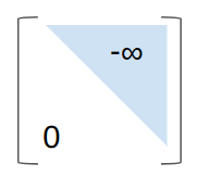
where \(\boldsymbol{M}\) is a lookahead mask with the upper right triangle set to negative infinity:

Check out this blog post for some additional nice coverage of self-attention masks.

Are We Done Yet?

Alright, we’ve got our baby transformer and we’ve added lookahead attention. Are we done?

Well, sort of. This is the minimum amount of stuff necessary to appropriately learn something that can call itself a transformer and that will probably sort-of work. All of the concepts are there. A real transformer will be the same, just bigger.

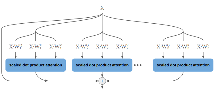
First, it will use multi-headed rather than single-headed attention. This just means that it does single-headed attention multiple times in parallel:

We could do that by running a \(\texttt{for}\) loop over multiple attention heads, but in practice it can be implemented by splitting our tensor into a new dimension according to the number of heads:

function (mha::MultiHeadAttention)(
    Q_in::Array{Float32, 3}, # [dim × ntokens × batch_size]
    K_in::Array{Float32, 3}, # [dim × ntokens × batch_size]
    V_in::Array{Float32, 3}, # [dim × ntokens × batch_size]
    mask::Array{Float32, 2}) # [ntokens × ntokens]

    dims = size(Q_in)
    dim = dims[1]

    # All matrices end up being [dim × ntokens × batch_size]
    Q = mha.q_proj(Q_in) # [dim × ntokens × batch_size]
    K = mha.k_proj(K_in) # [dim × ntokens × batch_size]
    V = mha.v_proj(V_in) # [dim × ntokens × batch_size]

    # Reshape to # [dim÷nheads × nheads × ntokens × batch_size]
    Q = reshape(Q, dim ÷ mha.nheads, mha.nheads, dims[2:end]...)
    K = reshape(K, dim ÷ mha.nheads, mha.nheads, dims[2:end]...)
    V = reshape(V, dim ÷ mha.nheads, mha.nheads, dims[2:end]...)

    # We're going to use batched_mul, which operates on the first 2 dimensions.
    # We want Q, K, and V to act as `nheads` separate attention heads, so we 
    # need to move the 'nheads' dimension out of the first 2 dimensions.
    Kp = permutedims(K, (3, 1, 2, 4)) # This effectively takes care of the transpose too
    Qp = permutedims(Q, (1, 3, 2, 4)) ./ √Float32(dim)
    logits = batched_mul(Kp, Qp) # [ntokens × ntokens × nheads × batch_size]

    # Apply the mask
    logits = logits .+ mask # [ntokens × ntokens × nheads × batch_size]

    # Compute the activations
    α = softmax(logits, dims=1) # [ntokens × ntokens × nheads × batch_size]

    # Run dropout on the activations
    α = mha.dropout(α) # [ntokens × ntokens × nheads × batch_size]

    # Multiply by V, again with a batched_mul
    Vp = permutedims(V, (1, 3, 2, 4))
    X = batched_mul(Vp, α)
    X = permutedims(X, (1, 3, 2, 4)) # [dim÷nheads × nheads × ntokens × batch_size]
    X = reshape(X, :, size(X)[3:end]...) # [dim × ntokens × batch_size]

    # Compute the outward projection
    return mha.out_proj(X) # [dim × ntokens × batch_size]
end

Note that in this code, the inputs are all X in the first multi-headed attention layer of the output head, whereas in the second one (called the cross attention layer), the queries Q_in are set to X whereas the keys and values are set to the output of the input head.

The other thing that a real transformer has is multiple transformer layers. That is, we repeat what we currently have as our input head and output head multiple times:

The Attention is All You Need paper used 8 parallel attention layers (attention heads) and 6 identical layers each in the encoder (input head) and decoder (output head).

Conclusion

I hope this post helps demystify the transformer architecture. They are the workhorse of modern large-scale deep learning, and its worth familiarizing yourself with them if you’re going to be working in that area. While complicated at first glance, they actually arise from fairly straightforward principles and solve some fairly practical and understandable problems. The information here should be enough to get started using them, or even roll your own from scratch.

Happy coding!