This post is an update on the sidescroller project. In short, I still find the project interesting, and as long as that is true, I want to work toward my original goal of a 2D sidescroller with arbitrary level geometry (i.e., not based on tiles or AABBs). I’ve achieved my stated goal of learning how to use the GPU and roll my own skeletal animation system, but I obviously haven’t built a game. A full game was, and still is, out of the question, but it would be cool to have something with a game loop and perhaps a complete level and a boss.

Fleshing out the game further requires fleshing out more of the game-play design. As such, physics must happen.

This blog post covers how I’m going about collision detection and resolution for convex polygons.

The Problem

We wish to simulate objects moving around in a 2D space. While we might eventually have fancy objects like ropes, let’s start by restricting ourselves to convex polygons:

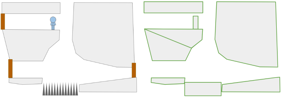
A crude rendition of a 2D platformer scene (left) and the convex polygons in it (right).

As we can see, nonconvex polygons can be represented by multiple convex polygons, so this isn’t all that restrictive.

Most of the polygons will be static. The floors and ceilings, for the most part, do not move. Entities like the player, monsters, eventual ropes, crates, etc. will need to move. That movement needs to obey the laws of physics, which mainly means integrating accelerations into velocities, velocities into positions, and handling collisions.

More formally, we have a scene comprised of \(m\) rigid bodies, some of which are static and some of which are dynamic. Each rigid body is defined by a convex polygon and a 2D state. Each convex polygon is represented as a list of vertices in counter-clockwise (right-hand) order:

More serious implementations might include additional information, like precomputed edge normals or an enclosing axis-aligned box for broad-phase collision detection, but let’s leave those optimizations out for now. And yes, I could have used an std::vector but I like having trivially copyable types since I’m serializing and deserializing my levels to disk and I don’t want to think too hard when doing that.

I made the simplification of keeping track of static bodies separately from dynamic rigid bodies. For the static bodies, the polygon vertices are directly defined in the world frame. For the dynamic bodies, the polygon vertices are defined in the body frame of the entity, and are then transformed according to the entity’s state:

A vertex \(\boldsymbol{v}\) in the body frame of a polygon can be transformed into the world frame according to:

\[\begin{bmatrix}v_x \\ v_y\end{bmatrix}_\text{world} = \begin{bmatrix}\cos \theta & -\sin \theta \\ \sin \theta & \hphantom{-}\cos \theta\end{bmatrix}\begin{bmatrix}v_x \\ v_y\end{bmatrix}_\text{body} + \begin{bmatrix}p_x \\ p_y\end{bmatrix}\]

As the physics evolve, these states change, but the polygons do not. In every frame, we’ll accumulate forces and torques on our bodies and use them to update the state. We’ll also have to perform collision detection and handle any resulting forces and torques.

State Propagation

We need to simulate the laws of motion. That is, solve \(F = m \> a\) and compute

\[\begin{matrix}v(t + \Delta t) = v(t) + \int a(t) \> dt \\ p(t + \Delta t) = p(t) + \int v(t) \> dt \end{matrix}\]

except in 2 dimensions with torques and rotations.

We can’t do exact integration, so we’ll have to rely on approximations. Games tend to run at pretty high frame rates, so its reasonable to approximate the update across a single frame using the Euler method:

\[\begin{align} u(t + \Delta t) &= u(t) + a_x(t) \Delta t \\ v(t + \Delta t) &= v(t) + a_y(t) \Delta t \\ \omega(t + \Delta t) &= \omega(t) + \alpha(t) \Delta t \\ x(t + \Delta t) &= x(t) + u(t) \Delta t \\ y(t + \Delta t) &= y(t) + v(t) \Delta t \\ \theta(t + \Delta t) &= \theta(t) + \omega(t) \Delta t\end{align} \]

or written a bit more compactly:

\[\begin{align} u’ &= u + a_x \Delta t \\ v’ &= v + a_y \Delta t \\ \omega’ &= \omega + \alpha \Delta t \\ x’ &= x + u \Delta t \\ y’ &= y + v \Delta t \\ \theta’ &= \theta + \omega \Delta t\end{align} \]

Apparently, doing this would work okay, but using symplectic Euler integration is a bit more stable. It uses the updated velocities for the position update:

\[\begin{align} u’ &= u + a_x \Delta t \\ v’ &= v + a_y \Delta t \\ \omega’ &= \omega + \alpha \Delta t \\ x’ &= x + u’ \Delta t \\ y’ &= y + v’ \Delta t \\ \theta’ &= \theta + \omega’ \Delta t\end{align} \]

Our physics system will perform this update for every dynamic body in every game tick. After doing so, it needs to handle collisions.

Properly handling collisions is a whole big field and there is potentially a lot to talk about. In an ideal sense, if we were to identify a collision, we’d back up in time to where the collision first occurred, and handle it there. That’s more accurate, but also complicated. In a scene with a bunch of objects and a bunch of collisions, we don’t want to be sorting by a bunch of collision times.

Instead, I’ll be taking inspiration from Verlet integration and enforce constraints via iteration. A single tick of the physics system becomes:

void PhysicsEngine::Tick(f32 dt) {
    // Euler integration
    for (auto& rigid_body : rigid_bodies_) {
        EulerIntegrationStep(&rigid_body.state, dt);
    }

    for (int i = 0; i < 4; i++) {
        EnforceConstraints();
    }
}

We’re running Euler integration once, then running several iterations of constraint enforcement! This iterative approach helps things shake out because oftentimes, which you resolve one constraint, you start violating another. Its a pretty messy way to do things, but its so simple to implement and can be surprisingly robust.

What constraints will we enforce? For now we’re only going to prevent polygons from interpenetrating. In general we can enforce a bunch of other types of constraints, most notably joints between bodies.

Collision Detection

Alright, all that pretext to get to the meat and potatoes of this post.

In order to prevent our rigid bodies from interpenetrating, we need to detect when they collide:

We can do this in a pairwise manner, only considering the world-space polygons of two rigid bodies at once.

We start by observing that two polygons are in collision if they share an interior. While that may be technically true, it doesn’t really tell us how to efficiently compute intersections.

A more useful observation is that two polygons A and B are in collision if

A contains any vertex of B, or
B contains any vertex of A, or
any edge in A intersects any edge in B.

This definition actually works for nonconvex as well as convex polygons (but don’t ask me about degenerate polygons that self-intersect and such). Unfortunately, its a bit inefficient. If A has \(n\) vertices and B has \(m\) vertices, then we’d be doing \(n+m\) polygon–point collision checks and then \(nm\) edge intersection checks. If we keep our polygons simple then it isn’t all that bad, but there are better methods.

One go-to method for 2D polygon collision checking is the separating axis theorem, which states that if two convex polygons A and B are in collision, then you cannot draw a line between them. (Sometimes these things seem kind of obvious in retrospect…):

We can draw a separating line between the two polygons on the left, but cannot for the colliding ones on the right.

One direct consequence of the separating axis theorem is that if you can draw a separating line, then the projection of each shape perpendicular to that line will also have a gap:

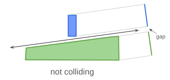
Similarly, if you project the two shapes in any direction that they cannot be separated in, then their projections will not have a gap:

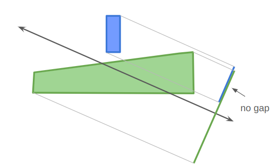
For convex polygons that are not colliding, a separating axis can always be constructed along one of the polygon’s edges. That is great — it means we only need to consider \(m + n\) possible separating axes.

Our collision detection algorithm is thus:

project both polygons onto all edge normals
if there are any gaps, then they do not intersect
otherwise, they intersect

Projecting a polygon along an axis is pretty easy:

struct PolygonProjection {
    f32 lo;
    f32 hi;
};

Overlap ProjectPolygonAlongDirection(
    const ConvexPolygon& polygon,
    const Vec2f normal)
{
    PolygonProjection proj;
    proj.lo = std::numeric_limits<f32>::infinity();
    proj.hi = -std::numeric_limits<f32>::infinity();
    for (u8 i = 0; i < polygon.n_pts; i++) {
        const f32 d = Dot(normal, polygon.pts[i]);
        proj.lo = std::min(d, overlap.lo);
        proj.hi = std::max(d, overlap.hi);
    }
    return proj;
}

Notice that the direction we pass in is the edge normal, not the edge tangent. This is because the normal is used to measure the distance away from the separating axis.

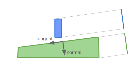
Two projects have a gap if proj_a.hi <= proj_b.lo || proj_b.hi <= proj_a.lo. Otherwise, they overlap.

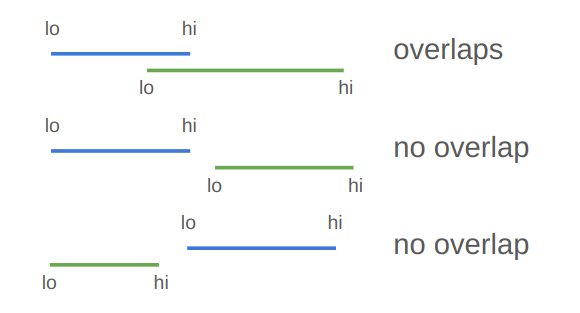
Our collision detection algorithm is thus:

bool CollidesInAnAxisOfA(
    const ConvexPolygon& A,
    const ConvexPolygon& B)
{
    Vec2f a1 = A.pts[A.n_pts-1];
    for (u8 i = 0; i < A.n_pts; i++) {
        const Vec2f& a2 = A.pts[i];
        const Vec2f tangent = Normalize(b - a);
        const Vec2f normal = Rotr(tangent);
 
        PolygonProjection proj_a = 
        ProjectPolygonAlongDirection(A, normal);
        PolygonProjection proj_b = 
             ProjectPolygonAlongDirection(B, normal);
        if (proj_a.hi > proj_b.lo && proj_b.hi > proj_a.lo) {
            return true; // no gap, thus a collision
        }
    }
}

bool Collides(
    const ConvexPolygon& A,
    const ConvexPolygon& B)
{
   return CollidesInAnAxisOfA(A, B) || CollidesInAnAxisOfA(B, A);
}

Penetration Vectors

Once we have determined that two polygons are colliding, we need to separate them. In order to do that, we need to find the penetration vector, or the shortest vector that can be added to one of the polygons such that they no longer overlap:

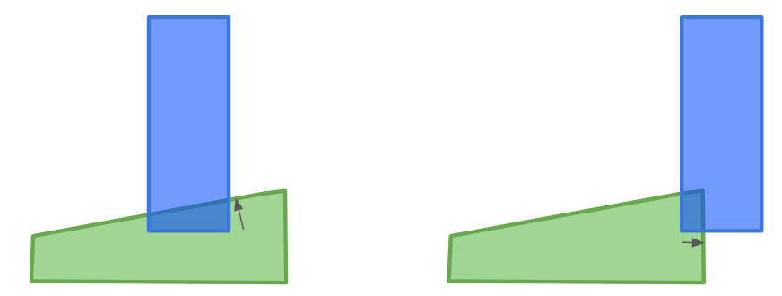
Rather than figuring this out from scratch, let’s modify our collision-checking routine to also figure this out.

When we project the two polygons into a direction, then the overlap of their projections is the distance we would need to move them in the projection direction to separate them:

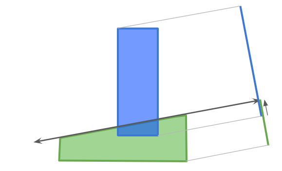
We can thus find the penetration vector by keeping track of the smallest overlap among all of the projections we do!

struct CollisionResult {
    bool collides;   // whether there is a collision
    f32 penetration; // the length of the penetration vector
    Vec2f dir;       // the unit penetration direction
}

// A helper function that projects along all of the edge tangents of A.
void CollisionHelper(
    const ConvexPolygon& A,
    const ConvexPolygon& B,
    CollisionResult* retval)
{
    Vec2f a1 = A.pts[A.n_pts-1];
    for (u8 i = 0; i < A.n_pts; i++) {
        const Vec2f& a2 = A.pts[i];
        const Vec2f tangent = Normalize(b - a);
        const Vec2f normal = Rotr(tangent);
        
        PolygonProjection proj_a = 
            ProjectPolygonAlongDirection(A, normal);
        PolygonProjection proj_b = 
            ProjectPolygonAlongDirection(B, normal);
        if (proj_a.hi > proj_b.lo && proj_b.hi > proj_a.lo) {
            retval.collides = true;
            return; // no gap, thus a collision
        }

        // Keep track of the smallest penetration
        f32 penetration = min(
            abs(proj_a.lo - proj_b.hi),
            abs(proj_a.hi - proj_b.lo))
        if (penetration < retval.penetration) {
            retval.penetration = penetration;
            retval.dir = normal;
        }
    }
}

CollisionResult Collides(
    const ConvexPolygon& A,
    const ConvexPolygon& B)
{
   CollisionResult retval = {};
   retval.penetration = std::numeric_limits<f32>::infinity();
   CollisionHelper(A, B, &retval);
   if (retval.collides) return retval;
   CollisionHelper(B, A, &retval);
   return retval;
}

Collision Manifolds

Our collision resolution logic can separate the polygons, but that isn’t enough to get realistic physics. We want to affect more than just their positions, but also their velocities and angular states. A collision should result in an impulse force that changes each body’s velocity and angular acceleration.

The torque is the counter clockwise force times the radius to the rigid body’s center of mass. That means we need the radius, which means knowing where the force is applied. So far we’ve only calculated the penetration normal, not where the penetration occurred.

Properly determining a collision response requires computing the contact point or contact manifold. Eric Catto has a nice GDC 2007 slide deck on this, but I wasn’t able to track down the actual talk that goes along with it, so it leaves something to be desired.

The contact manifold represents the points at which two objects come into contact. Ideally that would be the very first points that touch as two objects collide, but because of our discrete time steps, we have to work with partial overlaps:

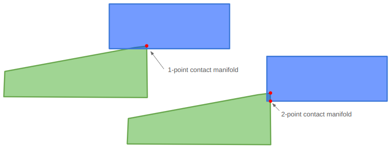
In some cases, a contact manifold should be an entire edge, but we’ll be approximating it using at most two points.

The contact manifold can be constructed using either polygon as a reference. We’ll be moving the polygons out of collision afterwards, so the contact manifold will be roughly the same independent of which polygon we choose:

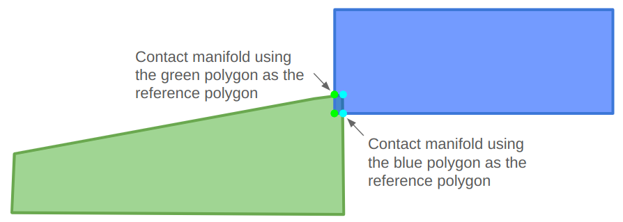
The reference polygon will be the one with the edge that the penetration vector is normal to. We’ll call that edge the reference edge. The other polygon is called the incident polygon, and we’ll need to identify an incident edge that crosses the reference edge.

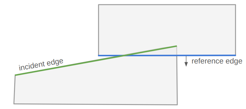
We will start by running our latest collision resolution algorithm, which gives us a penetration unit vector and magnitude. We have to slightly modify that code to keep track of which polygon it came from, so that we know which polygon is the reference polygon.

If it determines that there is no collision, we are done. Otherwise, we then identify the incident edge, which shall be the edge in the incident polygon whose outward normal is most opposed to the reference edge normal:

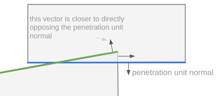
int inc_edge_index = 0;
int inc_edge_index_succ = 0;
f32 min_dot = std::numeric_limits<f32>::infinity();

int i_prev = I->n_pts - 1;
for (u8 i = 0; i < I->n_pts; i++) {
    common::Vec2f normal_i = Rotl(Normalize(I->pts[i] - I->pts[i_prev]));
    f32 dot = common::Dot(normal, normal_i);
    if (dot < min_dot) {
        min_dot = dot;
        inc_edge_index = i_prev;
        inc_edge_index_succ = i;
        }
    i_prev = i;
}

We then clip the incident edge to lie between the end caps of the reference edge:

This clipping is done in two steps — first by clipping the incident edge (which is a line segment) to lie on the negative side of the left halfspace and then again to lie on the negative side of the right halfspace. We can clip a line segment to a halfspace using the dot product of the endpoints with the halfspace normal vector (which is tangent to the reference edge) and comparing that to the dot product of the reference edge endpoint.

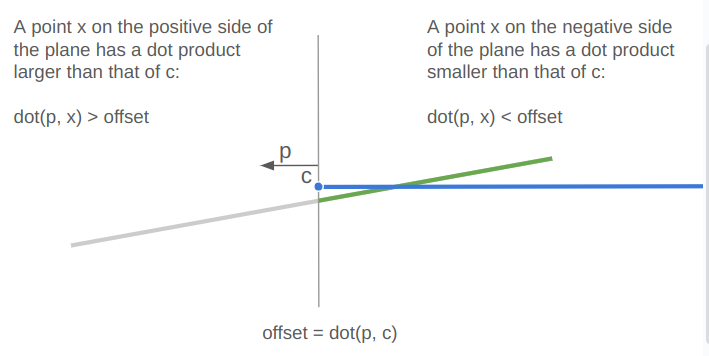
struct ClipResult {
   int n_pts;
   Vec2f pts[2];
};
ClipResult ClipSegmentToHalfspace(
    const Vec2f a,
    const Vec2f b,
    const Vec2f plane_normal,
    const f32 plane_offset,
    const int ref_edge_index) {

    ClipResult retval = {};

    // Compute the distances of the end points to the plane
    f32 dist_a = Dot(plane_normal, a) - plane_offset;
    f32 dist_b = Dot(plane_normal, b) - plane_offset;

    // If the points are on the negative side of the plane, keep them
    if (dist_a <= 0.0f) {
        retval.pts[retval.n_pts] = a;
        retval.n_pts += 1;
    }
    if (dist_b <= 0.0f) {
        retval.pts[retval.n_pts] = b;
        retval.n_pts += 1;
    }

    // If the points are on different sides of the plane, 
    // then we need to find the intersection point. 
    // (We don't have to do anything in the case that the
    // points are both on the positive side of the plane.)
    if (dist_a * dist_b < 0.0f) {
        // Keep the intersection points
        f32 interp = distance_0 / (distance_0 - distance_1);
        retval.pts[retval.n_pts] = a + interp * (b - a);
        retval.n_pts += 1;
    }

    return retval;
}

If we fully clip the segment away (which shouldn’t happen), then we don’t have a real intersection.

The collision manifold will consist of all endpoints in the clipped incident edge that penetrate across the reference edge. This explains how we can end up with either a 1- or a 2-point collision manifold. We can once again use a dot product and compare it to a base offset:

f32 face_offset = Dot(reference_normal, reference_a);
for (int i = 0; i < 2; i++) {
    // Get the distance of the ith endpoint along the normal from the
    // reference face. A negative value indicates penetration into the
    // reference polygon.
    f32 separation = Dot(reference_normal, clip.pts[i]) - face_offset;
    if (separation <= kEps) {
        manifold.points[manifold.n_pts] = clip.pts[i];
        manifold.n_pts += 1;
    }
}

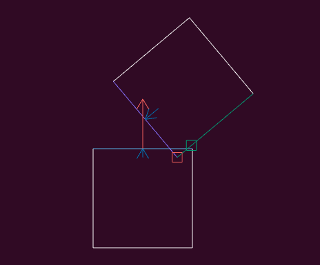
I coded up a visualization of this computation to help with debugging. The red vector is the unit normal along the reference edge, the little aligned blue vector is the same vector scaled by the penetration, the little red square is the 1 point in this collision manifold, and the little green square is the other endpoint of the clipped incident edge, which in this case was not accepted into the collision manifold:

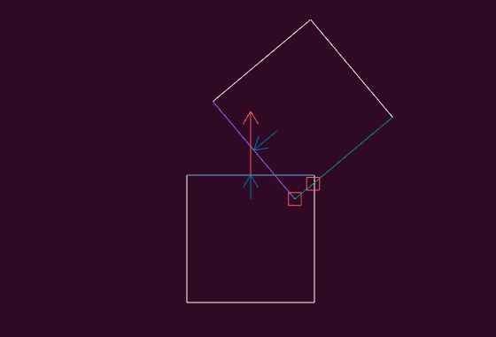
We can set up a case where there are two points in our collision manifold:

I can interact with my visualization by translating or rotation the one square around:

Collision Resolution

Now that we can detect collisions, calculate penetration vectors, and calculate a collision manifold, we can finally do the work of resolving a collision. Wikipedia has a good overview of this, but I’ll write it out here for good measure.

If we have a collision, then our contact manifold will contain one or two contact points. For starters let’s work with the case of a single contact point \(\boldsymbol{c}\). We’ll assume that body A is the reference polygon.

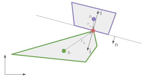
We can simulate the effect of a collision by imparting opposed impulses to the colliding bodies. This impulse is the integral of the force acting on each body over that collision timestep.

The impulse force depends on the relative velocity between the two objects. Let \(\boldsymbol{r}_A\) and \(\boldsymbol{r}_B\) be the vectors from each body’s center of mass (usually its centroid) to the contact point. Then we can calculate the relative velocity at the contact point:

\[\boldsymbol{v}_\text{rel} = (\boldsymbol{v}_B + \omega_B \times \boldsymbol{r}_B) – (\boldsymbol{v}_A + \omega_A \times \boldsymbol{r}_A)\]

The impulse is zero if this relative velocity along the normal is positive.

The normal impulse for the objects is:

\[j = \frac{-(1+e)\boldsymbol{v}_\text{rel} \cdot \boldsymbol{n}}{\frac{1}{m_A} + \frac{1}{m_B} + \frac{(\boldsymbol{r}_A \times \boldsymbol{n})^2}{I_A} + \frac{(\boldsymbol{r}_B \times \boldsymbol{n})^2}{I_B}}\]

where \(e \in [0,1]\) is the coefficient of restitution that determines how elastic the collision is, \(m_A\) and \(m_B\) are the polygon masses, and \(I_A\) and \(I_B\) are their moments of inertia.

We then update each polygon’s linear and angular speed according to:

\[\begin{align} \boldsymbol{v}_A’ &= \boldsymbol{v}_A \> – \frac{j}{m_A} \boldsymbol{n} \\ \boldsymbol{v}_B’ &= \boldsymbol{v}_B + \frac{j}{m_B} \boldsymbol{n} \\ \omega_A’ &= \omega_A \> – \frac{j}{I_A} \left(\boldsymbol{r}_A \times \boldsymbol{n}\right) \\ \omega_B’ &= \omega_B + \frac{j}{I_B} \left(\boldsymbol{r}_B \times \boldsymbol{n} \right)\end{align}\]

When there are two points in the contact manifold, one might be tempted to approximate the collision with their mean. I found that that doesn’t quite work correctly in all cases. For example, in the situation below, the rotation causes the estimated contact point to move right, which imparts a torque in the wrong direction:

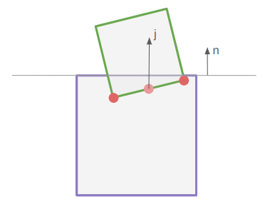
In order to fix this, I process both contact points, but weight the impulse in proportion to the penetration depth.

Positional correction is similar. To resolve the collision, we simply need to separate the two bodies along the penetration unit normal by a distance equal to the penetration \(\delta\). We could split the difference and shift the incident polygon by \(\delta / 2\) and the reference polygon by \(-\delta / 2\) along the normal, but we also want to account for their relative masses.

To account for the masses, we’d want to move the incident polygon by

\[\frac{\delta}{2} \frac{m_A}{m_A + m_B}\]

and the reference polygon by

\[-\frac{\delta}{2} \frac{m_B}{m_A + m_B}\]

where \(m_B\) is the mass of the incident polygon and \(m_A\) is the mass of the reference polygon. The heavier polygon is moved less.

However, as stated earlier, rather than fully resolve the collision, we will perform multiple, smaller resolution steps. If our penetration has a magnitude \(\delta\), we only apply \(\beta \delta\) where \(\beta\) is between 0 and 1, typically something like 0.4. We move the incident polygon in the penetration normal direction by that amount, and the reference polygon by the opposite amount. This will help jostle multiple conflicting collisions in a nice way such that they hopefully find a stable, valid solution.

For a nice code reference for all this, I recommend Randy Paul’s Impulse Engine.

Conclusion

And that’s enough to get us some pretty solid solid-body physics!

We actually did quite a lot in this post. We set off to do polygon collision resolution, started with polygon intersections, realized we also needed to figure out the penetration vector, did that, and then realized that to get appropriate impulses we needed to compute approximate collision manifolds. We then used that information to compute impulses, apply them, and to physically separate any colliding bodies.

We don’t have any friction. Its actually pretty easy to add, but I figured this post was already long enough.

We haven’t yet talked about any sort of spatial partitioning or other broad-phase collision tactics. No special memory allocation strategies, stable contact points, or joints. As always, there is a whole world of potential complexity out there that can be tackled if and when its needed, and we want to tackle it.

I highly recommend the Box2D repo as a helpful reference. It is a bit more mature, which can lead to some excessive complexity, but on the whole it is actually very cleanly written and extremely well documented.

Happy coding.

Tim Wheeler

2D Collision Detection and Resolution