DeepMind’s AlphaGo made waves when it became the first AI to beat a top human Go player in March of 2016. This version of AlphaGo – AlphaGo Lee – used a large set of Go games from the best players in the world during its training process. A new paper was released a few days ago detailing a new neural net—AlphaGo Zero—that does not need humans to show it how to play Go. Not only does it outperform all previous Go players, human or machine, it does so after only three days of training time. This article will explain how and why it works.

Monte Carlo Tree Search

The go-to algorithm for writing bots to play discrete, deterministic games with perfect information is Monte Carlo tree search (MCTS). A bot playing a game like Go, chess, or checkers can figure out what move it should make by trying them all, then checking all possible responses by the opponent, all possible moves after that, etc. For a game like Go the number of moves to try grows really fast.
Monte Carlo tree search will selectively try moves based on how good it thinks they are, thereby focusing its effort on moves that are most likely to happen.

More technically, the algorithm works as follows.  The game-in-progress is in an initial state s0, and it is the bot’s turn to play. The bot can choose from a set of actionsA. Monte Carlo tree search begins with a tree consisting of a single node fors0. This node is expanded by trying every actiona∈A and constructing a corresponding child node for each action. Below we show this expansion for a game of tic-tac-toe:

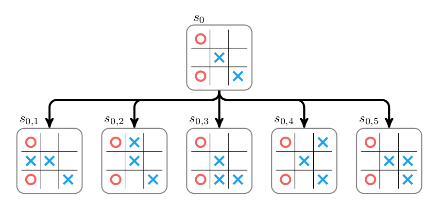
The value of each new child node must then be determined. The game in the child node is rolled out by randomly taking moves from the child state until a win, loss, or tie is reached. Wins are scored at \(+1\), losses at \(-1\), and ties at \(0\).

The random rollout for the first child given above estimates a value of \(+1\). This value may not represent optimal play-it can vary based on how the rollout progresses. One can run rollouts unintelligently, drawing moves uniformly at random. One can often do better by following a better-though still typically random-strategy, or by estimating the value of the state directly. More on that later.

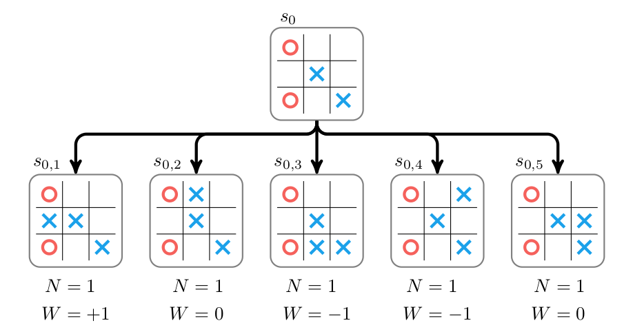
Above we show the expanded tree with approximate values for each child node. Note that we store two properties: the accumulated value \(W\) and the number of times rollouts have been run at or below that node, \(N\). We have only visited each node once.

The information from the child nodes is then propagated back up the tree by increasing the parent’s value and visit count. Its accumulated value is then set to the total accumulated value of its children:

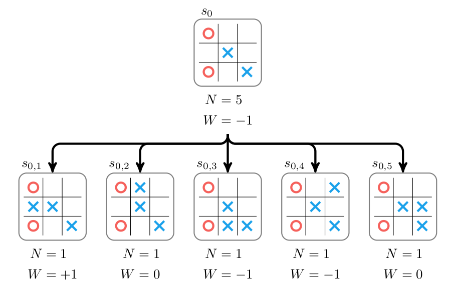
Monte Carlo tree search continues for multiple iterations consisting of selecting a node, expanding it, and propagating back up the new information. Expansion and propagation have already been covered.

Monte Carlo tree search does not expand all leaf nodes, as that would be very expensive. Instead, the selection process chooses nodes that strike a balance between being lucrative-having high estimated values-and being relatively unexplored-having low visit counts.

A leaf node is selected by traversing down the tree from the root node, always choosing the child \(i\) with the highest upper confidence tree (UCT) score:

$$U_i = \frac{W_i}{N_i} + c \sqrt{\frac{\ln N_p}{N_i}}$$

where \(W_i\) is the accumulated value of the \(i\)th child, \(N_i\) is the visit count for the \(i\)th child, and \(N_p\) is the number of visit counts for the parent node. The parameter \(c \geq 0\) controls the tradeoff between choosing lucrative nodes (low \(c\)) and exploring nodes with low visit counts (high \(c\)). It is often set empirically.

The UCT score (\(U\)’s) for the tic-tac-toe tree with \(c=1\) are:

In this case we pick the first node, \(s_{0,1}\). (In the event of a tie one can either randomly break the tie or just pick the first of the bet nodes.) That node is expanded and the values are propagated back up:

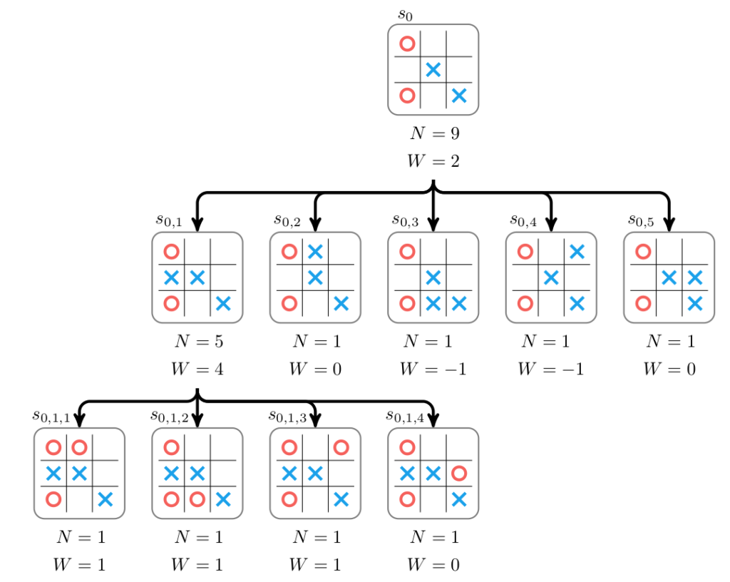
Note that each accumulated value \(W\) reflects whether X’s won or lost. During selection, we keep track of whether it is X’s or O’s turn to move, and flip the sign of \(W\) whenever it is O’s turn.

We continue to run iterations of Monte Carlo tree search until we run out of time. The tree is gradually expanded and we (hopefully) explore the possible moves, identifying the best move to take. The bot then actually makes a move in the original, real game by picking the first child with the highest number of visits. For example, if the top of our tree looks like:

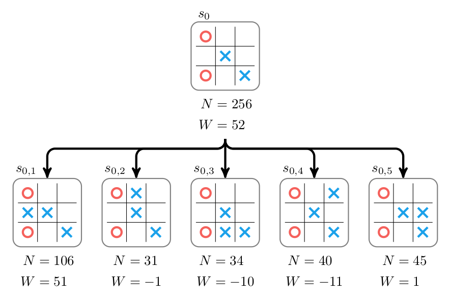
then the bot would choose the first action and proceed to \(s_{0,1}\).

Efficiency Through Expert Policies

Games like chess and Go have very large branching factors. In a given game state there are many possible actions to take, making it very difficult to adequately explore the future game states. As a result, there are an estimated \(10^{46}\) board states in chess, and Go played on a traditional \(19 \times 19\) board has around \(10^{170}\) states (Tic-tac-toe only has 5478 states).

Move evaluation with vanilla Monte Carlo tree search just isn’t efficient enough. We need a way to further focus our attention to worthwhile moves.

Suppose we have an expert policy \(\pi\) that, for a given state \(s\), tells us how likely an expert-level player is to make each possible action. For the tic-tac-toe example, this might look like:

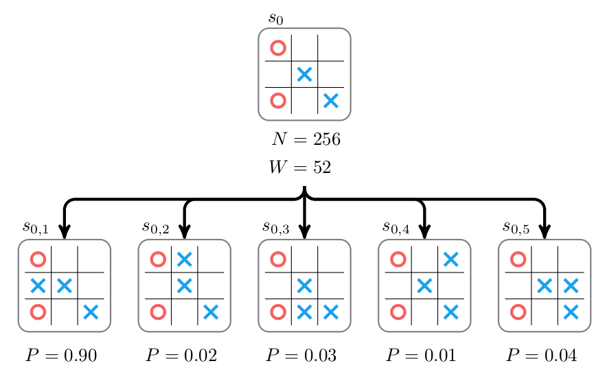
where each \(P_i = \pi(a_i \mid s_0)\) is the probability of choosing the \(i\)th action \(a_i\) given the root state \(s_0\).

If the expert policy is really good then we can produce a strong bot by directly drawing our next action according to the probabilities produces by \(\pi\) , or better yet, by taking the move with the highest probability. Unfortunately, getting an expert policy is difficult, and verifying that one’s policy is optimal is difficult as well.

Fortunately, one can improve on a policy by using a modified form of Monte Carlo tree search. This version will also store the probability of each node according to the policy, and this probability is used to adjust the node’s score during selection. The probabilistic upper confidence tree score used by DeepMind is:

$$U_i = \frac{W_i}{N_i} + c P_i \sqrt{\frac{\ln N_p}{1 + N_i}}$$

As before, the score trades off between nodes that consistently produce high scores and nodes that are unexplored. Now, node exploration is guided by the expert policy, biasing exploration towards moves the expert policy considers likely. If the expert policy truly is good, then Monte Carlo tree search efficiently focuses on good evolutions of the game state. If the expert policy is poor, then Monte Carlo tree search may focus on bad evolutions of the game state. Either way, in the limit as the number of samples gets large, the value of a node is dominated by the win/loss ratio \(W_i / N_i\), as before.

Efficiency Through Value Approximation

A second form of efficiency can be achieved by avoiding expensive and potentially inaccurate random rollouts. One option is to use the expert policy from the previous section to guide the random rollout. If the policy is good, then the rollout should reflect more realistic, expert-level game progressions and thus more reliably estimate a state’s value.

A second option is to avoid rollouts altogether, and directly approximate the value of a state with a value approximator function \(\hat{W}(x)\). This function takes a state and directly computes a value in \([-1,1]\), without conducting rollouts. Clearly, if \(\hat{W}\) is a good approximation of the true value, but can be executed faster than a rollout, then execution time can be saved without sacrificing performance.

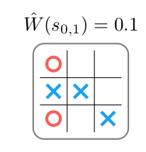
Value approximation can be used in tandem with an expert policy to speed up Monte Carlo tree search. A serious concern remains-how does one obtain an expert policy and a value function? Does an algorithm exist for training the expert policy and value function?

The Alpha Zero Neural Net

The Alpha Zero algorithm produces better and better expert policies and value functions over time by playing games against itself with accelerated Monte Carlo tree search. The expert policy \(\pi\) and the approximate value function \(\hat{W}\) are both represented by deep neural networks. In fact, to increase efficiency, Alpha Zero uses one neural network \(f\) that takes in the game state and produces both the probabilities over the next move and the approximate state value. (Technically, it takes in the previous eight game states and an indicator telling it whose turn it is.)

$$f(s) \rightarrow [\vec p, W]$$

Leaves in the search tree are expanded by evaluating them with the neural network. Each child is initialized with \(N = 0\), \(W = 0\), and with \(P\) corresponding to the prediction from the network. The value of the expanded node is set to the predicted value and this value is then backed up the tree.

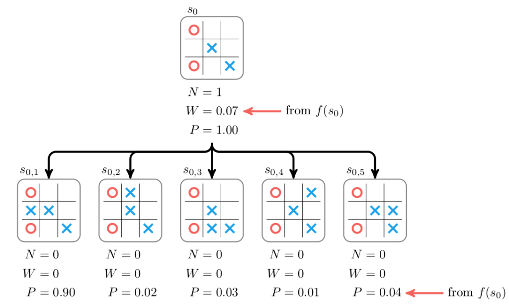
Selection and backup are unchanged. Simply put, during backup a parent’s visit counts are incremented and its value is increased according to \(W\).

The search tree following another selection, expansion, and backup step is:

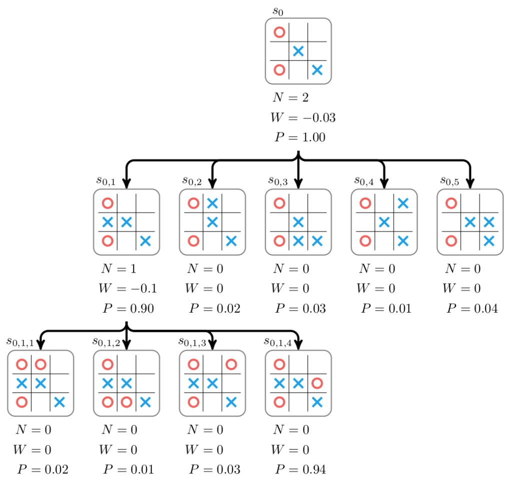
The core idea of the Alpha Zero algorithm is that the predictions of the neural network can be improved, and the play generated by Monte Carlo tree search can be used to provide the training data. The policy portion of the neural network is improved by training the predicted probabilities \(P\) for \(s_0\) to match the improved probability \(\vec \pi\) obtained from running Monte Carlo tree search on \(s_0\). After running Monte Carlo tree search, the improved policy prediction is

$$\pi_i = N_i^{1/\tau}$$

for a constant scalar \(\tau\). Values of \(\tau\) close to zero produce policies that choose the best move according to the Monte Carlo tree search evaluation.

The value portion of the neural network is improved by training the predicted value to match the eventual win/loss/tie result of the game, \(Z\). Their loss function is:

$$(W-Z)^2 + \vec \pi^\top \ln \vec p + \lambda \|\vec \theta\|_2^2$$

where \((W-Z)^2\) is the value loss, \( \vec \pi^\top \ln \vec p\) is the policy loss, and \(\lambda \|\vec \theta\|_2^2\) is an extra regularization term with parameter \(\lambda \geq 0\) and \(\vec \theta\) represents the parameters of the neural network.

Training is done entirely in self-play. One starts with a randomly initialized set of neural network parameters \(\vec \theta\) are then improved by using gradient descent (Or any of the more sophisticated accelerated descent methods-Alpha Zero used stochastic gradient descent with momentum and learning rate annealing.) on the loss function for a random selection of states played.

Closing Comments

And that’s it. The folks at DeepMind contributed a clean and stable learning algorithm that trains game-playing agents efficiently using only data from self-play. While the current Zero algorithm only works for discrete games, it will be interesting whether it will be extended to MDPs or their partially observable counterparts in the future.

It is interesting to see how quickly the field of AI is progressing. Those who claim we will be able to see the robot overlords coming in time should take heed – these AI’s will only be human-level for a brief instant before blasting past us into superhuman territories, never to look back.