I recently became interested in the Thousand Brain Theory of Intelligence, a theory proposed by Jeff Hawkins and the Numenta team about how the human brain works. In short, the theory postulates that the human neocortex is made up of on the order of a million cortical columns, each of which is a sort of neural network with an identical architecture. These cortical columns learn to represent objects / concepts and track their respective locations and scales by taking in representations of transforms and producing representations of transforms that other cortical columns can use.
This post is not about the Thousand Brain Theory, but instead about the sub-architectures used by Numenta to model the cortical columns. Numenta was founded back in 2005, so a fair bit of time has passed since the theory was first introduced. I read through some of their papers while trying to learn about the theory, and ended up going back to “Why Neurons have Thousands of Synapses, a Theory of Sequence Memory in the Neocortex” by Hawkins et al. from 2016 before I found a comprehensive overview of the so-called hierarchical temporal memory units that are used in part to model the cortical columns.
In a nutshell, the hierarchical temporary memory units provide a means of having a local method for learning and allows individual neurons to become very good at recognizing a wide variety of patterns. Hierarchical temporal memory is supposedly good at robust sequence recognition and better models how real neurons work.
Real Neurons
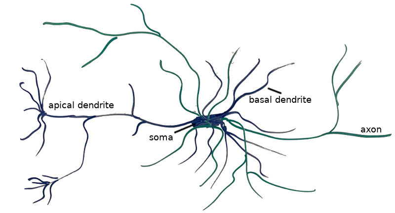
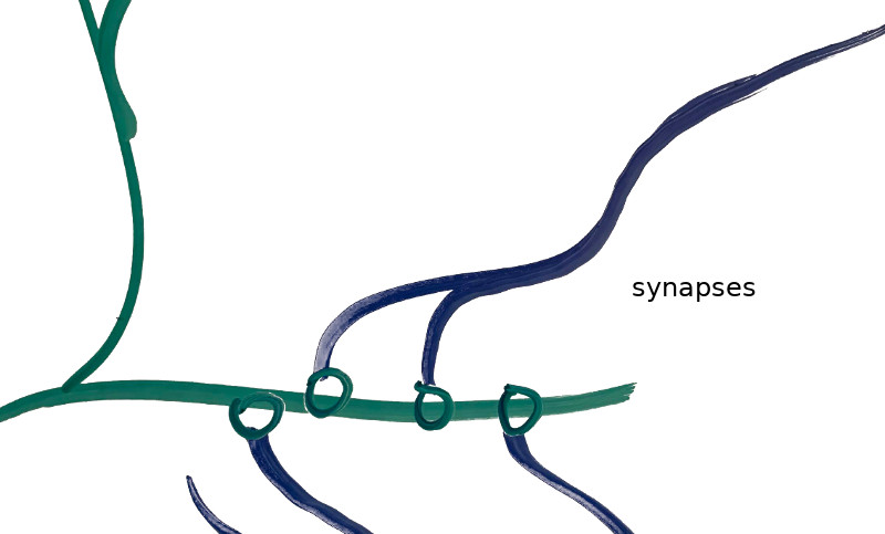
The image above shows my crude drawing of a pyramidal cell, a type of cell found in the prefrontal cortex. The Thousand Brains Theory needs a way to model these cells. The thick blob in the center is the cell soma, or main body of the cell. The rest are connective structures that allow the neuron to link with other neurons. The dendrites (blue) are the cell’s inputs, and receive signals from other cells and thereby trigger the cell to fire or prepare to fire. The axons (green) are the cell’s outputs, and propagate the charge produced by a firing cell to the dendrites of other neurons. Dendrites and axons connect to one another via synapses (shown below). One neuron may have several thousand synapses.
Real neurons are thus tremendously more complicated than is typically modeled in a traditional deep neural network. Each neuron has many dendrites, and each dendrite has many potential synaptic connections. A real neuron “learns” by developing synaptic connections. “Good” connections can be reinforced and made stronger, whereas “bad” connections can be diminished and eventually pruned altogether.
Each dendrite is its own little pattern matcher, and can respond to different input stimuli. Furthermore, different dendrites are responsible for different behavior. Proximal dendrites carry input information from outside of the layer of cells, and if they trigger, they cause the entire neuron to fire. Basal dendrites are connected to other cells in the same layer, and if they trigger, they predispose it to firing, causing it to fire faster than it normally would, thus preventing other neurons in the same region from also firing. (Apical dendrites are not modeled this this paper, but are thought to be like basal dendrites but carry feedback information from higher layers back down.)
Neurons in Traditional Deep Learning
It is interesting to see how much simpler a neuron is in traditional deep learning. There, a single neuron merely consists of an activation function, such as ReLU or sigmoid, and acts on a linear combination of inputs:
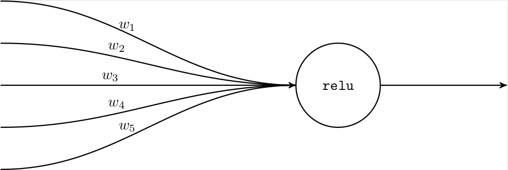
Mathematically, given a real input vector \(x\), the neuron produces a real output \(\texttt{relu}(x^\top w)\). Representing a neuron in memory only requires storing the weights.
This representation is rather simplified, and abstracts away much of the structure of the neuron into a nice little mathematical expression. While the traditional neural network / deep learning representation is nice and compact (and differentiable), the hierarchical temporal model introduced by Hawkins et al. models these pyramidal neurons with much greater fidelity.
In particular, the HTM paper claims that real neurons are far more sophisticated, capable of learning to recognize a multitude of different patterns. The paper seeks a model for sequence learning that produces neural models that excel at online learning, high-order prediction, multiple simultaneous predictions, continual learning, all while being robust to noise and not require much tuning. That’s quite a tall order!
Neurons in the HTM Model
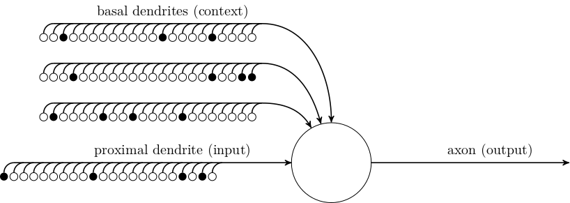
HTM neurons are more complicated. In this model, each cell has \(1\) proximal dendrite that provides input from outside of the cell’s layer, and \(B\) basal dendrites that provide contextual information from other neurons in the same layer. Each dendrite has some number of synapses that connect it to the axons of other neurons. The figure above shows 22 synapses on each dendrite, will filled circles showing whether the connected axon is firing or not.
In the HTM model, a dendrite activates when a sufficient number of its synapses are active. That is, if at least \(\theta\) connected neurons that it has synaptic connections with fire. If we represent the a dendrite’s input as a bit-vector \(\vec d\), then the dendrite activates if \(\|\vec d\|_1 \geq \theta \).
An HTM cell can be in three states. It is normally inactive. If its proximal dendrite activates, then the cell becomes active and fires, producing an output on its axon. If a basal dendrite activates, then the cell becomes predictive, and if it becomes active in the next time-step, it will fire faster than its neighbors and prevent them from firing. We reward basal dendrites that cause the cell to become predictive before activation, and we punish dendrites that don’t. In this way, learning (for basal dendrites at least) is entirely local.
A dendrite can “learn” by changing its synaptic connections. In a real cell, a synapse can be reinforced by growing thicker / closer to its axon. A more established synapse is more permanent and harder to remove. In the HTM model, we maintain a set of \(K\) potential synapses per neuron. Each potential synapse has a scalar “permanence” value \(0 \leq p \leq 1\) that represents its state of growth. A value close to 0 means the synapse is unformed; a value larger than a connection threshold (\(p \geq \alpha\)) means the synapse is established and activation of the neighbor cell will contribute to firing of the dendrite, and a value close to 1 means the synapse is well established.
At least three observations can be made at this point. First, notice that we only care about the binary firing state of neurons: whether they are active or not. We have thus already deviated from the traditional continuous representations used in deep learning.
Secondly, the thresholded firing of behavior of dendrites is similar to a traditional activation function (especially a sharp sigmoid) in the sense that below a threshold, the dendrite does nothing, and above the threshold it fires. The paper claims that this behavior adds robustness to noise. If \(\theta = 10\) and we have connections to 12 active neurons for a certain repeated input, but one of the 12 fails to fire, then we’ll still trigger.
Thirdly, representing a single HTM neuron requires more computation and memory. In particular, representing the basal dendrites requires \(B K\) permanence values, and each neuron has three possible states, and we need to keep track of what the previous state was in order to trigger learning.
Layers and Mini-Columns
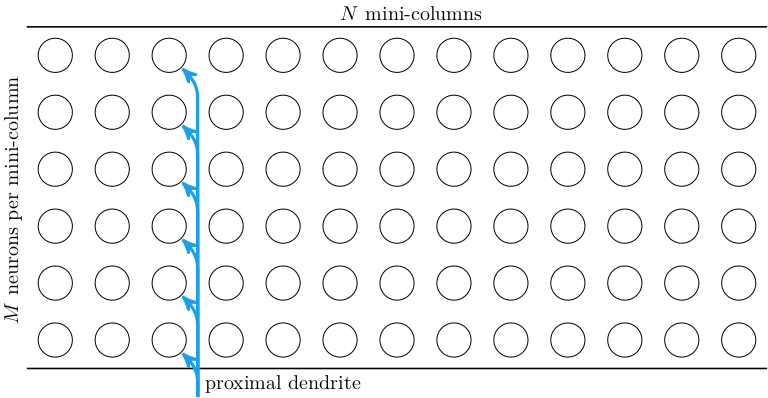
The cells in the HTM model are arranged in layers. The paper only concerns itself with a single layer at a time. Each layer consists of \(N\) mini-columns of neurons, each with \(M\) neurons. Each neuron has one proximal dendrite, whose input comes from outside of the layer. All neurons in a mini-column share the same proximal dendrite input:
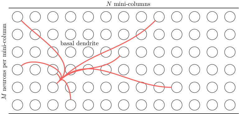
Each neuron has \(B\) basal dendrites that have up to \(K\) synapses to other cells in the same layer. A single basal dendrite for a single cell is shown below. (Note that, technically speaking, the basal dendrite is not directly connected to the soma of the other cells, but has synapses that connect it to the axon of each connected cell.)
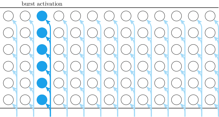
The proximal dendrites are responsible for getting the neuron to become active. The neurons in each mini-column share the same proximal dendrite input. If a proximal dendrite becomes active, it can cause all neurons in that mini-column to become active. This is called a burst activation:
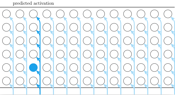
The basal dendrites are responsible for predicting whether the neuron will become active. If a basal dendrite becomes active, due to enough of its connected cells being active, it will cause the cell to enter the predictive state:

inhibit them and prevent then from firing. In the HTM model, if there is a proximal activation, any predictive cells become active first. We only get a burst activation if no cells are predictive. Thus, when inputs are predicted (ie learned), we get sparse activation:
As such, the learned synaptic connections in the basal dendrites are what allow the neuron to predict activation patterns. Initially, inputs will not be predicted, and burst activations will trigger entire mini-columns. This increases the chance that basal dendrites will activate, which will increase the number of predictions. Accurate predictions will be reinforced, and will lessen the number of overall activations. Over time, a trained network will have very few burst activations, perhaps only when shifting between two different types of input stream contexts.
Learning
The learning rule is rather simple. A predicted activation is reinforced by increasing the strength of synaptic connections in any basal dendrite that causes the predictive state. We decrease all permanence values in that dendrite by a small value \(p^-\) and increase all permanence values of active synapses by a larger, but still small value \(p^+\). This increases the chance that a similar input pattern will also be correctly predicted in the future.
In an unpredicted activation, (i.e. during a burst activation), we reinforce the dendrite in the mini-column that was closest to activating, thereby encouraging it to predict the activation in the future. We reinforce that dendrite with the same procedure as with predicted activations.
We also punish predictions that were not followed by activations. All permanences in dendrites that causes the predictive state are decreased by a small value slightly smaller than \(p^-\). (I used \(p^-/2\).)
Constant Input
We can see this learning in action, first on a constant input stream. I implemented the HTM logic and presented a simply layer with a constant input stream with some random fluctuations. This experiment used:
M = 3 # number of cells per minicolumn
N = 5 # number of minicolumns
B = 2 # number of basal dendrites per cell
K = 4 # number of potential synapses per cell
α = 0.5 # permanence threshold for whether a synapse is connected
θ = 2 # basal dendrite activation threshold
p⁻ = 0.01 # negative reinforcement delta
p⁺ = 0.05 # positive reinforcement delta
A single training epoch in this very simple experiment consists of a single input. The Julia source code for this, and the subsequent experiment, is available here.
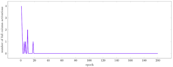
As we expect, the layer to starts off with many burst activations, and gradually has no burst activations as training progresses:
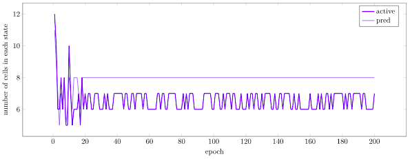
If we look at the number of cells in each state, we see that initially we get a lot of active and predictive cells due to the many burst activations, but then gradually settle into a stable smaller number of each type:
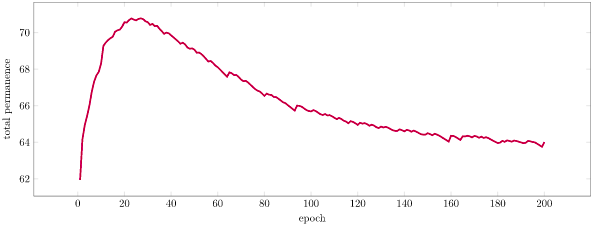
We can also look at total network permanence over time. We see an initial increase in permanence as we develop new synaptic connections in order to predict our burst activations. Then, as we being to correctly predict and activations become sparser, we shrink our synapses and lose permanence:
Sparsity and Multiple Simultaneous Predictions
The authors stress the importance of sparsity to how hierarchical temporal memory operates. The paper states:
We want a neuron to detect when a particular pattern occurs in the 200K cells [of its layer]. If a section of the neuron’s dendrite forms new synapses to just 10 of the 2,000 active cells, and the threshold for generating an NMDA spike is 10, then the dendrite will detect the target pattern when all 10 synapses receive activation at the same time. Note that the dendrite could falsely detect many other patterns that share the same 10 active cells. However, if the patterns are sparse, the chance that the 10 synapses would become active for a different random pattern is small. In this example it is only 9.8 x 10⁻²¹.
In short, sparsity lets us more accurately identify specific predictions. If sequences are composed of input tokens, having a sparse activation corresponding to each input token lets us better disambiguate them.
The other advantage of sparse activations is that we can make multiple predictions simultaneously. If the layer gets an ambiguous input that can cause two different possible subsequent inputs, the layer can simply cause both predictions to occur. Input sparsity means that these multiple simultaneous predictions can be present at the same time without a great chance of running into one another or aliasing with other predictions.
Note that this sparsity does come at the cost of requiring more space (as in memory allocation), something that the paper does not venture much into.
Sequence Learning
As a final experiment, I trained a layer to recognize sequences. I tried to reproduce the exact same experimental setup as the paper, but that was allocating about 1.6Gb per layer, which was way more than I wanted to deal with. (The permanences alone require \(4 B M N K\) bytes if we use float32’s, and at \(B = 128\), \(M = 32\), \(N = 2048\), and \(K = 40\) that’s 1,342,177,280 bytes, or about 1.3 Gb). This experiment used:
M = 8     # number of cells per minicolumn
N = 256   # number of minicolumns
B = 4     # number of basal dendrites per cell
K = 40    # number of potential synapses per dendrite
α = 0.5f0 # permanence threshold for whether a synapse is being used
θ = 2 # basal dendrite activation threshold
p⁻ = 0.01 # negative reinforcement delta
p⁺ = 0.05 # positive reinforcement delta
I trained on 6-input sequences. I generated 20 random sparse inputs / tokens (4 activations each), and then generated 10 random 6-token sequences. Each training epoch presented each sequence once, in a random order.
Below we can see how the number of burst activations decreases over time. Note that it doesn’t go to zero – burst activations are common transitions between sequences.
The paper presented prediction accuracy. I am not certain what they meant by this – perhaps the percentage of times that a neuron entered a predictive state prior to an activation, or the number of activations for which at least a single neuron was predictive. I chose to consider the “prediction” of the neural network to be a softmax distribution over tokens. I had the probability of the next token bitvector \(\vec t\) be proportional to \(\texttt{exp}(\beta (\vec \pi \cdot \vec t))\) for \(\beta = 2\). Here \(\vec \pi\) is the bitvector of predicted columns, i.e. \(\pi_i\) is true if mini-column \(i\) has at least one cell in a predictive state. Anyways, I felt like this measure of prediction accuracy (i.e. mean likelihood) more closely tracked what the layer was doing and how well it was performing. We can see this metric over time below:
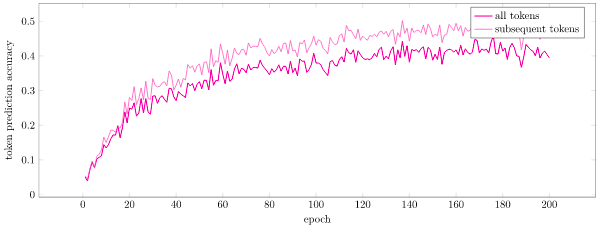
Here we see that the layer is able to predict sequences fairly well, hovering at about 50% accuracy for tokens that are not the first token (we transition to a random 6-token sequence, so its basically impossible to do well there), and about 40% accuracy across all tokens. I’d say this is pretty good, and demonstrates the proof of concept of the theory in practice.
Conclusion
Overall, hierarchical temporal memory is a neat way to train models to recognize sequences. Personally, I am worried about how much space the model takes up, but aside from that the model is fairly clean and I was able to get up and running very quickly.
he paper did not compare against any other substantial sequence learners (merely a dumb baseline). I’d love for a good comparison to something like a recurrent neural network to be done.
I noticed that the HTM only trains dendrites that become predictive (or chooses dendrites in the case of a burst activation). This requires the mini-column of the parent neuron to be activated in order to be trained. If a certain column is never activated, the dendrites for that neuron will not be trained. Similarly, if some dendrite is not really used, there is a very low chance it will ever be used in the future. I find this to be a big waste of space and an opportunity for improvement. We are, in a sense, building a random network in initialization and hoping that some of the connections work out, and ignoring the rest. This random forest approach only gets us so far.
I had a lot of fun digging into this and noodling around with it. I am very excited about the prospect of human-level cognition, and maybe something HTM-like will get us there some day.